SOVIET VOROSHILOV ACADEMY LECTURES
PRACTICAL LESSONS

LESSON III: TACTICAL AND OPERATIONAL CALCULATIONS

1. General: In this three hour lesson the students will become familiar with Soviet mathematical approaches to decision making. They will consider a series of specific problems isolated from tactical situations and focus on the formulas, nomograms, tables, and other technical aids for calculations. The problems will be seen again in tactical and operational settings in the later practical exercises.


2. Sublesson Introduction: Stress to the students that these three hours will probably be the most arcane for them of all in the course. They have just seen that Soviet headquarters and staffs perform the same functions as do U.S. staffs, even if in a somewhat different organizational structure. In the past hour they learned that Soviet commanders have a formal method for insuring that every bit of relevant information is considered while making decisions, but the Soviet estimate of the situation is not that much different from the U.S. method. However, in this class on mathematical calculations they will find that the Soviet officers will want to "scientifically substantiate" every part of their decisions if at all possible. Since the Soviet view is that troop control is itself the science of forecasting the outcome of future events, mathematics plays a larger role in Soviet planning procedures than in the US methods. However, the mathematics involved is quite simple and straight forward. Most of the formulas involve basic algebra. A few employ probability theory or logarithms, but even these are not difficult to understand.


3. Teacher Learning Objective: Develop basic ability of students to perform standard calculations using nomograms, formulas, and norms in accordance with typical Soviet practice to prepare them for roles of commander, chief of staff, and chief of operations at division, army, and front levels.


Task: Explain Soviet mathematical methods for calculating various tactical and operational factors of interest to the commander. Demonstrate the equations, nomograms, and tables used when making these calculations. Give the students an opportunity to practice and test their proficiency at this by leading them through the solution of a series of simple calculations.

Condition: Given student reading assignment and class handouts.

Standard: The students should be able to perform typical Soviet calculations in support of combat decisions. They should understand the use of nomograms and tables. If there is time to discuss the concepts behind the creation of nomograms they should be encouraged to design their own to solve other practical problems. Since all these problems can be solved with desk top computers, the students should consider developing programs to do this work, especially by using spreadsheets.


4. Level of Instruction: Familiarization.


5. Method of Instruction: Lectures, discussion, and practical exercises.


6. Author's Intent:

The most important result is that the students should be able to embrace the Soviet mathematical approach while they take the role of Soviet staff officer in the OPFOR headquarters. This is the area in which their American ways of doing things will be most difficult to overcome. The purpose of this three hour class is to reduce feelings either of being threatened by mathematics or of considering it unnecessary busywork. In the context of the real work currently required of the OPFOR staff it is quite possible to get away without using the level of mathematics based planning taught in this course. Consequently there will considerable reluctance to dig in and really become adept at the use of these methods. In the future we will provide computer based solutions, which will bypass the use of most nomograms. Nevertheless, the students can't really "think Red" without getting into the spirit of the Soviet mathematical approach to combat.

This class is based on Chapter Five of the Handbook. The students should have a copy of this and should have read it prior to class. A representative sample of the types of calculations found in that chapter has been selected for presentation in this class. The instructor should lead the students through one iteration of the problem solving the equation, moving through the nomogram step by step, or filling in the table, etc. as required. Then he should give them a similar example and ask them to solve it in a few minutes. A spot check and discussion of the answers will provide an indication of their success in understanding the material. The problems are presented in the same sequence as they are shown in the Handbook, since that was deemed an appropriate organization. The formulae and nomograms are contained in Chapter 5 of the Handbook. No times are shown for the individual problems, since these will no doubt vary with the instructor's and students' interest.

The lecture notes contain information on a wider variety of calculations performed by the staff during the decision making process and during the course of combat. The instructor may discuss these as well. Some will be studied during other courses on planning of other functions such as reconnaissance or artillery.


7. Equipment/Materials: viewgraphs, handouts for calculations.


8. Homework: None.

OUTSIDE READING:

Handbook on Soviet Staff methods, Chapter Five.
Vayner, Tactical Calculations.
Donnelley, et.al. The Sustainability of Soviet Army in Battle.


9. Annexes

Discussion agenda
Lesson notes
List of Viewgraphs

Operational and Tactical Calculations


1. Basic Time and Distance Calculation.

This is a generic and ubiquitous problem which appears also in many different formulations and with embellishments to take more elaborate details into consideration. In this example we consider the time taken for halts and for moving into the new area. It is a good problem to familiarize the students with the use of nomograms. They can easily check their answers by solving the standard formula.


2. Calculation of Time to Begin Move to Start Line

This formula has a somewhat more limited application. It is required to establish the time a unit should leave its assembly area in order for the head of column to cross the initial line (point) at the appointed time. Since Soviet march orders give the latter time as the official time the commander must meet, he will have to perform this calculation in order to determine when he should get his unit underway. Again, the formula is simple enough that the students can check their use of the nomogram by solving the equation as well.


3. Calculation of Time to Deploy into a New Assembly Area

The purpose of this exercise is to determine how long it will take the march column to move into the assembly area when the length of the column is longer that the length of the area itself. This formula is needed because the calculation of the time required to make the march itself will be based on the head of the column reaching the further point while traveling at the march rate. After that time then the rest of the column must close up into the assembly area while moving at a lesser rate of march. The answer to this question is then entered into calculations of the kind shown in exercise 1.


4. Calculation of Time a Unit will be in a New Area

This exercise makes use of the method for solving problems by creating a standard table in which the user merely enters the appropriate data for the variables and follows the instructions for performing the mathematical calculations. The answer then appears in the given box. We have experimented with converting tables of this sort to computer spreadsheets with complete success.


5 Calculation of the Duration of a March from one Area to Another

This example combines the parts of the problem shown in the previous exercises into a single calculation. This is the more usual practical application of the formulas. The operations staff will make these calculations and report the results to the chief of staff and commander to insure that all subordinate formations and units are able to accomplish their moves on time.


6. Determine the Required Movement Rate for a Unit to Regroup in a New Area

This is the reverse calculation from the previous one. In this case the operations staff wants to find out what movement rates must be achieved in order to enable formations can reach new assembly areas within a designated time. If the rate seems beyond the achievable, then the distance to the new area should be reduced. Again, this equation can be solved by using a spread sheet and various options can be compared quickly.


7. Calculation of Length of Route, Average Speed, and Duration of Movement of Moving Column

This is one of the more complex applications of the basic movement equations. In this case the situation requires movement of the columns over a series of route segments having different characteristics which affect the rate of movement. This would typically come into play when the unit moved over highways, country roads, cleared dirt lanes, etc. The table provides a simple way to enter all the information is a fool proof manner and come out with the answer without having to memorize or even look at the underlying formulas.


8. Calculation of Overall Depth of Column Consisting of Several Sub-columns

The operations staff needs to know how much road space unit columns will occupy in order to clear that space from interference by other columns and in order to provide air defense and other protection. The rear service staff must do similar calculations for logistics columns. The equations are relatively simple to solve, but the nomogram is faster.


9. Calculation of Duration of Passage of Narrow Points and Difficult Segments

We have all experienced the phenomena of "accordioning" when a line of vehicles must get into "stop and go" traffic due to some obstacle. Obviously there will be many such obstacles to the free passage of combat formations and units. These equations take into account two different situations, which have different influences on the moving column. One is the case in which the length of the obstacle is very short. This imposes a kind of stop and go effect on the column as each vehicle in turn crosses the obstacle. The other case is one in which the length of the obstacle is longer than the length of the marching column. In this case the vehicles will not only slow briefly in sequence, but will move at a slower rate for a more prolonged distance before picking up speed again. Moreover, if the column is to maintain integrity, the lead vehicles cannot pick up speed to their maximum until the tail end vehicles have cleared the obstacle.


10 Calculation for Passage Times Across Start Point (SL) by the Head and Tail of the Column

The Soviet movement planners want to know not only when the head of each column will pass the start line and each other control point, but also when the tail of each column passes these points. This is so they can plan when cross traffic or other moving columns can pass the same point without interfering with the first column. The nomogram simplifies the work, but the formula is not difficult to apply either.


11. Calculation of Expected Time and Distance of Probable Point of Contact with Advancing Enemy

With this example we move from simple movement calculations to one of the most vital tactical and operational issues. The Soviet commanders are constantly concerned about forecasting when and where their formations and units will encounter enemy forces moving into contact. The practical applications of this equation come not only in the period of initial movement to contact at the initial stage of a campaign, but also frequently during the battle or engagement as first or second-echelons move into contact with enemy reserves. In the practical exercises for operations planning we will discuss what is done with the results of this calculation and how the Soviet commander will seek to influence the result to suit his concept for combat.


12. Calculation of Time Required for Advancing and Deploying Sub-units to Change From Line of March into the Attack

This is another vital tactical calculation that is also checked by the division and army staffs as well. The preferred Soviet style of attack is "from the march". In this method the artillery will have deployed forward into prepared positions and will be standing by to commence artillery preparatory fire. The Soviet way of coordinating combat keys on Che hour, the moment the first leading troops set foot in the first line enemy trench. Consequently all times for approach march and deployment and for supporting artillery fire must be calculated backwards from Che hour. The basic time and distance equation is simple, but in this case it must be applied for each segment of the march and deployment as the formation shifts from regimental to battalion, to company, to platoon columns and finally into the assault formation. Therefore the table provides a more convenient way to enter the relevant data and come out with the answer. Again, a spread sheet would be an even more convenient way to investigate a variety of options.


13. Calculation of the Time and Distance to the Line of Contact

The earlier example of time and distance equation did not take into consideration extra variables. In this example some of these are included. In particular, this table allows the staff to insert data for various delay times which may be inflicted on each side. The instructor can compare the equations and show how these variables are depicted in the formula. The table allows someone to enter the data without even seeing the equations.


14 Calculation of Expected Time and Rate of Overtaking when Pursuing the Enemy

We hope to find many opportunities to use this formula or nomogram. Obviously the computation is easier to perform than the actions which will, hopefully, lead to its use. In any event the nomogram is quite simple. We will use this formula in a tactical setting in later practical exercise to determine the time a forward detachment must reach a river to prevent a retreating enemy from establishing a defense there.

15. Calculation of the Work Time Available to the Commander and Staff for Organizing Repulse of Advancing Enemy Forces

Point out to the students the relevance of this problem to the Soviet staff, that is always operating in a forecasting mode. This exercise is particularly relevant for the superior staff that is trying to intervene with supporting measures to delay an enemy before it reaches the line of a subordinate unit. Or it can be used by a commander facing the arrival of an enemy at his own location and wanting to get his artillery or anti-tank units into action in time to stop the attack. The same principles would apply to create an equation to express the relationship between time to some future event and variables expressing the actions of actors on both sides.


16. Calculation of Length of Time to Operate Command Post in a Single Location

We skipped this example found in the handbook because of its simplicity, However, if the instructor wishes he can draw the students attention to it on page 5-79. The equation would be useful for any situation involving operation of some element in one place for a duration of time governed by the relative movement rate of the element and some other element having a different rate of movement.


17. Determination of Quantity of Various Weapons, Reconnaissance, Support, Communications etc. for Task Performance

This is a very useful equation. The nomogram is specific for a given set of data, but similar nomograms could be created for other data sets. Or the procedure could be developed on a computer. This is a good example of Soviet interest in forecasting by means of probabilities. The instructor should study pages 80-82 of the handbook thoroughly and perhaps read the sections of Vayner. If the instructor is uncomfortable with statistics and probabilities he might do some extra reading in the literature on this. The Soviet example, which we reproduce, makes use of a reconnaissance topic. For the student example the instructor can substitute other topics related to operations.


19. Calculation of Strike Capability of Sub-units

This is a very interesting problem taken from a recent Soviet article. The instructor may want to read the discussion on modeling battle on pages 5-83 to 86 and in Chapter One of the Handbook. This is an area still under investigation by Soviet theorists. The literature is quite dynamic, so instructors should watch for more developments. In this example the Soviet operations staff can relate the depth of penetration a unit might achieve to its combat potential and that of the enemy and to the expected casualties of both sides. The casualties would have to be calculated with other equations or from norms. We have extrapolated from the Soviet example to apply the equation for a full division.
This formula will be used again in a tactical setting in the practical exercises for division planning. This and subsequent exercises depend on the application of a Soviet system of combat potential scores "utils". We do not yet have a complete series of such scores for all weapons and units, but believe such information is available at FT. Leavenworth. The instructor should discuss the concept behind these scores with the students.


20. Calculation of the Width of Main Attack Sector

Determining the width of the main attack sector is certainly one of the most critical issues facing the Soviet commander. This equation appeared in a recent Soviet article. The equation is actually nothing more than basic algebra in which a proportion is stated in a way to facilitate solving for one of its elements. The instructor must emphasize that since it appeared in the literature it has been badly misused by various American commentators who apparently don't understand what constitutes the Soviet "Main attack" or "Strike" sector of a formation or how the commander determines how wide it should be.

The point of this equation is to provide a simple way to determine what the correlation of forces will be in a strike sector of given width when the overall correlation is such and such, or in reverse, how wide a strike sector might be when given various correlation of forces values overall and within the sectors. Thus it is a tool for finding out the stated answers. It is not used as the means for determining either what the proper correlation of forces should be nor what the most desirable width of main attack sector should be. In fact in our practical exercises we show that the answers one derives from using this equation should lead directly to considerations about what measures to undertake to change the obtained results so that both the sector width and the force correlations established by other be achieved.


21. Calculation of Required Destruction of Enemy

This calculation uses a variation of the same equation as the previous exercise. In this case a nomogram has been developed related to a specific set of loss data. Other nomograms would have to be created for other levels of losses. However, the use of this equation and method itself points to the Soviet concept for shifting the correlation of forces in their favor by employing air power, or artillery, or some other means of attacking the enemy or degrading his forces prior to or outside the confines of the combined arms battle. Thus it draws attention to the dynamic nature of the Soviet idea of correlations of forces.


22. Calculation of Rate of Advance in Relation to Correlation of Forces

That there is any direct correlation of rate of advance with correlation of forces is itself a controversial subject. Most commentators agree that many other factors enter into the real world situation and produce different outcomes. Nevertheless the desire to have some relatively simple way for forecasting the rate of advance that might be achieved under future combat conditions is overwhelming. In fact it is virtually essential to create plans which the development of the combat action centers around various subordinates reaching their mission lines at prescribed times. A simpler way to do this is to use more general norms based on historical and personal experience. In other words the commander could simply issue an order that the subordinate unit must reach a certain distance in so many hours based on his desires and "gut" feelings.

The instructor may discuss this and comment on the various American army attempts to come up with some relationship of advance rate and force ratios. We have skipped the next example in the Handbook, on determining losses in relation to both correlation of forces and rate of advance, but the instructor may want to bring up this example as well.

The nomograms found in the Handbook were developed by American officers on the basis of Soviet concepts, but they do not represent any official Soviet norms. They are useful as educational tools to illustrate the procedures. It is likely that Soviet staffs have this kind of data in computers and can run this kind of problem without using nomograms.


24. Determine the Required Amount of Manpower and Weapons for Bringing Sub-Units back up to Sufficient Strength to Restore their Combat Capability

This is a simpler calculation than it sound like. A table is provided to make the assembly and display of initial data even easier. The instructor should use the given data to fill out the table once and then let the students repeat the exercise using a different set of numbers.


25. Determine the Expected Radiation Dose

If the instructor is running out of time, he may want to skip this example. The issues are quite clear and the forms and nomogram relatively simple for the students to figure out themselves. We do not have any calculations on radiation in the planning exercises later in the course.

26 Calculation to Select the Optimal Travel Route

This is a very interesting Soviet example of using simple techniques to solve in approximate fashion what would be a more complex problem to solve rigorously. The commander is faces with a very real time constraint and the need to determine the optimum solution from among a number of various possible solutions. Using a computer now will allow for more accuracy.

The Soviet field method is to create a simple table and employ a kind of successive calculations to gradually build up the information on which to base the selected best solution.


29. Calculation to Determine the Effectiveness of Fire Destruction Means

Operational calculations

GENERAL

The Soviet planning process includes a great deal of time and effort in making detailed calculations. Therefore it is important for the students to learn the proper procedures for calculating a wide variety of information about both enemy and friendly forces. These calculations occur at each stage of the decision process.

CLARIFICATION OF THE MISSION

At this time the commander must calculate the depth and width of the formation (unit) missions, the time to achieve these and the required rate of advance. From these calculations he derives his general idea of the number of armies required and their echelonment and formation. He and/or the chief of staff must calculate the time available for planning and preparation of the troops for combat. From this they develop a time schedule for accomplishing all these needed actions.

ESTIMATE OF THE SITUATION

ENEMY

During this phase the commander first calculates the density of enemy forces in each different area and for various depths. He calculates the enemy nuclear capability in terms of the number of targets and kilotons it is possible for the enemy to deliver. He also calculates enemy artillery capabilities in terms of hectares of target per salvo, aircraft capabilities in terms of numbers of sorties per day and enemy air defense in terms of numbers of aircraft that can be shot down at one time.

The commander calculates the time and space factors, first those related to mobilizing and preparing the units for combat and then those that show when units can reach their combat starting locations. For these he includes the enemy operational and strategic reserves in order to establish how soon they will reach the areas he believes the enemy will want to assign to them. These calculations make use of simple rate of movement formulas and established norms for movement over various roads as well as norms for accomplishing each activity such as debarking, dismounting, deploying and etc. Next the calculations take into consideration the disturbances to the time schedules that might be introduced by disruptions to the line of communications, blocking of ports, destruction of air fields and other similar events.

The probable enemy concept of operations is assessed by estimating the length of delay actions he can achieve on each line based on the calcuation of the density of forces and means. If the density is one company per kilometer then a division can hold for a day or so within its 12 km deep position. At this time the possible locations at which the enemy reserves can intervene in the battle are noted from the calculation of when and from where they can launch counterattacks.

If the initial enemy position is to the rear of his prefered battle position, calculations are made to find out if a meeting engagement between the large units is to be expected.

FRIENDLY

When the commander turns to the estimate of friendly forces he makes many of the same calculations. First there is the movement from garrison including time to mobilize and bring the forces to full combat readiness and time to establish the unit attack groupings. These calculations are mostly reconfirmation of existing planned activities. The commander can turn to the staff all of whom know what will be asked of them ahead of time to insure that units can arrive on time. The calculations require information on the status of units, and where they draw supplies or how the supplies will be delivered.

The combat capability of friendly forces includes calculation of nuclear capability in kilotons and numbers of warheads, artillery firepower in hectares of target per salvo, air defense capability in numbers of aircraft destroyed and aircraft in squadron sorties per day. The air defense calculations are especially complex since they involve detailed numerical factors for each type of weapon and target acquisiton.

The commander must next establish the correlation of troops and means. This is shown in a table titled COMPOSITION OF FORCES AND DENSITY. The friendly and enemy forces are shown in terms of nuclear rounds, nuclear delivery means, divisions, artillery, tanks, antitank missiles, air defense weapons, and aircraft. The ratios are calculated using quantitative and qualitative factors and are figured for the formation (unit) as a whole and for each individual axis and for each relevant depth of mission. They are calculated for; the start of the operation, after the initial nuclear strike, at the end of the first day, at the end of the immediate mission of the armies, at the end of the immediate mission of the formation (unit) , and at the end of the subsequent mission of the formation (unit) .

The calculations for correlation and density for each of the points in time after the start involve calculations of the estimated losses that each side will have incured. The calculation for losses in the initial nuclear strike is made by taking the total number of rounds allocated (or estimated for the enemy) and from this the number and yield that will be targeted against divisions to get a number of rounds per division. Then norms are applied to estimate losses. One norm is that if a division is hit by more than 6 -7 nuclear rounds it suffers medium damage and is incapacitated. If it is hit by more than 12 rounds it is destroyed. The effect of losses is estimated and 30% is considered heavy casualties while 50 - 60% will equal destruction. Losses for each day of combat are calculated according to norms for conventional and nuclear warfare. The correlation at the end of the first day would include loss norms of about 5% for personnel and 8% for tanks and lesser numbers for other equipment. One norm is that in 7 days of fighting a loss of 50 - 80% for tanks is expected. Some other norms are for army level in conventional war 1.1 - 1.3 % personnel per day; for nuclear 3.8 - 5.3 % per day; and 7.7 - 10.4 for the entire operation in conventional war and 27 - 42 % for the entire operation in nuclear war. Equipment loss norms include conventional of 8-9% per day and 40 - 60 % for vehicles and 50 - 80 % for tanks. All these norms are used to calculate the correlation of remaining forces for the various subsequent times. For instance, at the end of 5 days in an operation it might be expected that the attacker will have suffered losses of 7% in personnel, 40% in tanks, 25% in APC and 35% in other vehicles while the defender will have suffered losses of 5% in personnel, 35% in tanks, 20% in APC and 30% in vehicles.

After both sides are calculated it is possible to make a deduction on the proper distribution of troops to the several axes and then to distribute the combat support arms and reserves, naval and airborne assaults and other support.
An important set of calculations is made for electronic warfare in determining how many communications links above division can be neutralized by the available REW assets. Each radio electronic warfare battalion has a capability based on its means to jam a certain number of radio nets of a certain power or type. The enemy can also jam certain links.

When the missions of the armies are determined there are then calculations related to the coordination of forces. These are to establish how groupings will be created and what times will be involved. A table showing who will do what at each time is prepared.

The locations and times for movement of the command posts are calculated based on the planned course of the offensive. Then the role of adjacent forces are considered. The calculations are made to see how the missions of adjacent forces might involve the formation (unit) and vice versa. For instance the time an airborne division can sustain itself before linkup with ground forces is used in calculating when the airborne operation should take place. One of the adjacent forces at the front level is the strategic rocket and air force. The timing of their strategic nuclear strike if any or the strategic air operation is considered in calculations on when to launch the operational strike.

TERRAIN

The terrain is then considered in calculations to refine the plans. The capacity of routes, ports, airfields, bridges, etc is considered to insure that the forces can move as planned. The economic situation in the theater is the basis for calculations on the availability of local resources such as supplies and transportation means.

CALCULATIONS DURING COMBAT

The staff accomplishes the following calculations during preparation for the operation and during break through of enemy defense:


Chief of operations directorate:
----- calculation on time required to prepare;
----- movement, deployment, beginning of attack of prepared defense, for the main forces of army (division);
(The movement norms for road march in rear areas in daylight is 30 km/hr and night 20 km/hr, but when near the enemy the rate drops to 10-15 km/hr. Near means at the distance for which enemy heavy artillery can fire or about 12-15 km. Also, the deployment itself requires 20-30 minutes.
----- determine the correlation of forces:
----- over the entire frontage;
----- on the main axis;
----- on other axes;
----- at the end of the first day of operation;
----- at time of repelling enemy counterattack;
----- at time of commitment of second=-echelon;
----- during water crossings;
(The correlation is done with help of the table list of forces and means.)
----- conduct of calculations on combat capabilities of forces during destruction of enemy forces; (total sum of hectares and of the number of targets that can be destroyed in fire preparation period.)
----- calculations on commandant's service, how much forces are needed to accomplish tasks;
( For total length of distance and number of roads add the number of men, sergeants, officers, APC radio stations etc. required).


Chief of reconnaissance:
----- calculations on enemy capabilities during his attack with nuclear strike on our forces;
----- (total destruction capability and (three elements - fire capability, movement capability, cover capability and support elements including supplies etc.)
----- calculations of enemy capabilities during attack with conventional means; same elements
----- calculation of enemy capability during counter attack:
----- calculate time required for enemy to prepare move, deploy, and the time for his attack; (time to prepare and move from garrison, time to travel on roads and deploy into combat time to prepare forces etc.)
----- calculate enemy forces and means able to conduct counter attack; (analysis of forces available from current locations in time expected)
----- calculate artillery fire capabilities during counter attack
----- calculation capabilities on friendly radio electronic combat reconnaissance units OSNAZ. (how many enemy targets they can discover and track at the same time) at what ranges.
----- calculation of capabilities of friendly radio-technical electronic combat reconnaissance units OSNAZ. (
----- calculation of SPETZNAZ reconnaissance companies. time area targets to find etc. (per day recon 2 targets for each patrol in area of 10 by 10 km.
----- calculation capabilities of air reconnaissance; (how many targets at what ranges how fast how many aircraft are available their technical capabilities


Chief of artillery:
----- calculation time for preparation, movement, deployment, and taking up artillery positions and prepare to open fire;
----- calculation on various artillery reconnaissance;
----- calculation various on artillery strikes in support of forward detachments and main forces;
----- calculations on density of artillery in the break through sector;
----- calculation and analysis of enemy defense (quantity of platoon strong points in forward line and in depth, artillery and mortar batteries, command posts, forces in second-echelon, reserves, positions of air defense rockets and units, anti-tank means and others)
----- calculation on organization of army, division, and regimental artillery groups.
----- calculations on fire capabilities of artillery;
----- calculation on capabilities of missile forces using nuclear, chemical, and conventional rockets. (
----- calculation of time for artillery preparatory fire, fire strikes, (means for preparatory fire) calculation on ammunition supplies; (
----- calculation on artillery support fire (strikes and barrages) and ammunition required;
----- calculation on anti-tank means and direct fire weapons during preparatory fire;
----- determine fire capability of the anti-tank reserve during repelling enemy counter-attack;
----- calculation on movement and shifting positions for artillery;


Commander of air forces (at front, or air representative at army)
----- calculation on air forces
----- calculation of fire capability of air forces during break through and during operation;
----- calculation of fire capability of helicopters during repelling enemy counter-attack;
----- calculation of fire capability of air forces during air support fire and accompanying fire;
----- calculation on time for preparation of air flights and movement and strikes in various levels of combat readiness against targets located in enemy rear areas;
----- calculation on repelling enemy air strikes by fighter aviation;
----- calculation various on air reconnaissance;
----- calculation on aerial photography;
----- calculation on delivery of reports about reconnaissance to the command post;


Chief of PVO:
----- calculation on combat capabilities of PVO forces of army during repelling mass enemy strikes and individual or small group strikes, during day and night and bad weather poor visibility conditions;( What area can be covered against air strike time to prepare numbers of rockets ready to fire
----- calculation on capabilities for observation and reconnaissance against enemy air forces; and warning forces;
----- calculation on repelling strikes by enemy by fighter aircraft at various levels of combat readiness and those on combat air patrol;


Chief of engineers:
----- calculation on engineer forces capabilities during opening lanes in mine fields;
----- capabilities of engineers during construction of mine fields;
----- calculation on creation of trenches strong points, cover for machines and vehicles, command points, etc.
calculation on engineer forces on opening column routes and roads in various terrain conditions;


Chief of radio electronic combat:
----- capabilities of radio units SPETZNAZ during jamming enemy radio electronic means;number of targets - they have designated capabilities and range and time for shift from one target to another - depends on training and on capability for recon to find targets to jam)
----- calculation of capabilities of radio technical units SPETZNAZ during covering forces from enemy direct bombardment; and maskirovka diversion of rockets etc.


Chief of chemical:



The staff performs the following calculations during repelling enemy sudden initial attack:
----- time enemy may be ready to attack and move deploy and strike with main forces;
----- enemy artillery capabilities aviation, and nuclear means;
----- time for preparation and open fire by artillery, rockets and aviation on enemy while moving forward;
----- calculation on combat capabilities of army forces;
----- correlation of forces and means in general and on each axis;


Staff calculations during meeting engagement:
----- calculation on location preparation, movement, deployment, and seizing the line of contact for the meeting engagement;
----- calculation on determining line for meeting the enemy in various conditions;
----- calculation on enemy combat capabilities;
----- calculation on preparation, movement, deployment, and attack by army main forces;
----- calculation on preparation, march, deployment, and occupation of firing positions and start of artillery fire strike on enemy;
----- calculation on combat capabilities of army forces;
----- correlation of fores of the sides in general and on each axis;


Staff performs similar calculations on repelling enemy counter-attack:

Staff calculations on commitment of second-echelon into engagement:
----- calculation on enemy combat capability;
----- calculation on preparation accomplish march, deployment, and enter engagement by second-echelon;
----- calculation of combat capability of army forces'
----- calculation on commandant service;
----- calculation analysis of enemy defense
----- calculation on time for preparatory fire and fire strikes, and ammunition supplies;
----- calculation on fire support and accompanying fire;
----- calculation on determination of anti-tank reserve capabilities;
----- calculation of capabilities mobile obstacle detachments to cover flanks;
----- calculation on density of artillery per km of front;
----- calculation on organization of artillery groups in division and regiments;
----- calculation on building routes by engineers;
----- calculation on opening lanes in enemy mine fields if any.
----- and others.


Staff calculations on forcing water obstacles:
----- calculation time for movement and deployment of forward detachments and forcing river by forward detachment.
----- calculation of time for movement, deployment, preparation, and forcing water obstacles by first echelon of army;
----- calculation on river crossing equipment for bridges, rafts, assault crossings, and swimming crossing;
----- calculation for creation of roads to crossing sites.
----- calculation on commandant's service in area of crossing with engineer forces;
----- calculation on organization of commandant's service by combined arms units and sub units during approach to crossing site.
----- calculation on fire capability of artillery, missile units PVO and combined arms formations;
----- calculation of capability of engineers for creating of bridges, fords and assault crossings.
----- calculation on preparation and flight crossing and seizing enemy bank by air assault operation.
----- calculation of combat capability of air forces to delay approaching enemy forces;
----- calculation of combat capability of fighter aviation to repel enemy air attack on crossing, by combat air patrol and air forces at air fields.


Staff also performs calculation of preparation and movement of command posts during the operation.

VG1 - Introduction and outline of Lesson III

VG2 - Basic time and distance calculation

VG3 - Basic time and distance calculation

VG4 - Nomogram - time and distance calculation

VG5 - Example basic time and distance

VG6 - Calculation of time to begin move to start line

VG7 - Calculation of time to begin move to start line

VG8 - Nomogram - time to begin move to start line

VG9 - Example - time to begin move

VG10 - Calculation of time to deploy into a new assembly area

VG11 - Calculation of time to deploy into a new assembly area

VG12 - Nomogram - time to deploy into new area

VG13 - Example - time to deploy in new area

VG14 - Calculation of time unit arrives in a new area

VG15 - Table Calculation of time unit arrives in a new area

VG16 - Blank table Calculation of time unit arrives in a new area

VG17 - Calculation of time unit arrives in a new area

VG18 - Example - time unit arrives in a new area

VG19 - Calculation of the duration of a march from one area to another

VG20 - Table calculation of duration of march

VG21 - Blank table calculation of duration of march

VG22 - Calculation of the duration of march from one area to another

VG23 - Example - duration of march

VG24 - Determine the required movement rate for a unit to regroup in a new area

VG25 - Form for calculating required travel speed

VG26 - Blank form for calculating required travel speed

VG27 - Determine the requried movement rate for a unit to regroup in a new area

VG28 - Example - required movement rate

VG29 - Calculation of length of route, average speed and duration of movement of moving column

VG30 - Form for calculation of transit time over multisegment route

VG31 - Blank form for calculation of transit time over multisegment route

VG32 - Calculation of transit time over multisegment route

VG33 - Example - transit time over multi-segment route

VG34 - Calculation of overall depth of column consisting of several sub-columns

VG35 - Nomogram - calculation of total length of column

VG36 - Calculation of overall depth of column consisting of several sub-columns

VG37 - Example - total depth of column

VG38 - Calculation of duration of passage of narrow points and difficult segments

VG39 - Nomogram - duration of passage of narrow point or obstacle

VG40 - Calculation of duration of passage of narrow points and difficult segments

VG41 - Duration of passage of narrow points and difficult segments (2)

VG42 - Duration of passage of narrow points and difficult segments (3)

VG43 - Duration of passage of narrow points and difficult segments (4)

VG44 - Duration of passage of narrow points and difficult segments (5)

VG45 - Example - duration of passage of obstacle

VG46 - Example - duration of passage of obstacle (2)

VG47 - Example - duration of passage of obstacle (3)

VG48 - Nomogram time to surmount long obstacle

VG49 - Calculation for passage times across start point (sl) by the head and tail of the column

VG50 - Calculation for passage times across start point (sl) by the head and tail of the column

VG51 - Nomogram - time to cross start or control point

VG52 - Calculation for passage times across start point (sl) by the head and tail of the column (2)

VG53 - Example time to pass point

VG54 - Calculation of expected time and distance of point of contact with advancing enemy

VG55 - Calculation of expected time and distance of point of contact with advancing enemy

VG56 - Nomogram - calculation of time and distance to point of contact

VG57 - Example - calculation time and distance of point of contact with advancing enemy

VG58 - Solution - calculation time and distance of point of contact with advancing enemy

VG59 - Calculation of time required for advancing and deploying sub-units to change from line of march into the attack

VG60 - Calculation of time required for advancing and deploying sub-units to change from line of march into the attack

VG61 - Table calculation of time to advance and deploy

VG62 - Calculation of the time and distance to the line of contact

VG63 - Table - calculation of expected time and distance to probable line of meeting engagement

VG64 - Blank table - calculation of expected time and distance to probable line of meeting engagement

VG65 - Calculation of the time and distance to the line of contact

VG66 - Example - the time and distance to the line of contact

VG67 - Calculation of expected time and rate of overtaking when pursuing the enemy

VG68 - Calculation of expected time and rate of overtaking when pursuing the enemy

VG69 - Calculation of expected time and rate of overtaking when pursuing the enemy (2)

VG70 - Nomogram - expected time and rate of overtaking enemy

VG71 - Example - expected time and rate of overtaking when pursuing the enemy

VG72 - Example - expected time and rate of overtaking when pursuing the enemy (2)

VG73 - Example - expected time and rate of overtaking when pursuing the enemy (3)

VG74 - Calculation of the work time available to the commander and staff for organizing repulse of advancing enemy forces

VG75 - Calculation of the work time available to the commander and staff for organizing repulse of advancing enemy forces

VG76 - Nomogram - work time available to commander and staff

VG77 - Example - work time available to the commander and staff for organizing repulse of advancing enemy forces

VG78 - Example - work time available to the commander and staff for organizing repulse of advancing enemy forces (2)

VG79 - Determination of quantity of various means for task performance

VG80 - Determination of quantity of various means for task performance

VG81 - Determination of quantity of various means for task performance

VG82 - Determination of quantity of various means for task performance

VG83 - Determination of quantity of various means for task performance

VG84 - Nomogram - quantity of weapons and probibility to fulfill task

VG85 - Determination of quantity of various means for task performance (2)

VG86 - Example - quantity of means for task performance

VG87 - Example of quantity of various means for task performance (2)

VG88 - Modeling battle

VG89 - Coefficients of comensurability

VG90 - Modeling battle

VG91 - Modeling battle

VG92 - Calculation of strike capability of sub-units

VG93 - Calculation of strike capability of sub-units

VG94 - Example of strike capability of sub-units

VG95 - Calculation of the width of main attack sector

VG96 - Calculation of the width of main attack sector

VG97 - Example of the width of main attack sector

VG98 - Calculation of required destruction of enemy

VG99 - Calculation of required destruction of enemy

VG100 - Nomogram - required destruction graph

VG101 - Example - of required destruction of enemy

VG102 - Calculation of rate of advance in relation to correlation of forces

VG103 - Nomogram - F factor and correlation of forces

VG104 - Example - rate of advance in relation to correlation of forces

VG105 - Nomogram - Force attrition army

VG106 - Nomogram - Force attrition front

VG107 - Determine the required amount of manpower and weapons for bringing sub-units back up to sufficient strength to restore their combat capability

VG108 - Form for calculation of required amount of forces

VG109 - Blank form for calculation of required amount of forces

VG110 - Determine the required amount of manpower and weapons for bringing sub-units back up to sufficient strength to restore their combat capability

VG111 - Example - the required amount of manpower and weapons for bringing sub-units back up to sufficient strength to restore their combat capability

VG112 - Determine the expected radiation dose

VG113 - Determine the expected radiation dose

VG114 - Nomogram - determine expected radiation dose

VG115 - Determine the expected radiation dose

VG116 - Example - the expected radiation dose

VG117 - Form for calculation of expected radiation dose

VG118 - Form - Quantitative characteristics of alternative routes

VG119 - Form - Effectrivenewss of artillery fire damage

VG120 - Form Effectiveness of artillery fire damage II

VG121 - Calculation to determine the effectiveness of fire destruction means

VG122 - Form for calculating weapons effectiveness

VG123 - Calculation to determine the effectivenss of fire destruction means

VG124 - Example - determine the effectiveness of fire destruction means

Operational and Tactical Calculations


1 Basic Time and Distance Calculation

Example problem using nomogram: Calculate the duration of a move along a 80 km route with an average speed of 35 km/hr, duration of halts total 1 hr & 30 min, and time taken to deploy into new area is 30 min.

Solution: Start at the 80 point on the bottom scale "Length of March" go up to the "Speed of movement -35 kph" line then horizontally across to the I line. Draw a line from that point to the II line passing through the .5 point on the "Pulling in" line, then another line downwards from the II line passing through 1.5 on the "Duration of halts" line. This intersects the "Duration of march" line at 4 hrs and 20 min.



Example problem using nomogram: Calculate the duration of a move along a ___ km route with an average speed of ___ km/hr, duration of halts total _________, and time taken to deploy into new area is ___min.

Solution: Start at the 80 point on the bottom scale "Length of March" go up to the "Speed of movement -_____ kph" line then horizontally across to the I line. Draw a line from that point to the II line passing through the ____ point on the "Pulling in" line, then another line downwards from the II line passing through _____ on the "Duration of halts" line. This intersects the "Duration of march" line at __________.



2 Calculation of Time to Begin Move to Start Line


Example problem: Determine the starting time for a column when the time for the head of the column to pass the start line is planned for 2100 hrs, the distance to the start line is 9 km, and the rate of march while moving out is 15 kph.

Solution:


Example using nomogram (Figure 83):

Using the same initial data as the previous example enter the nomogram on the X axis at 9 km move up to 15 kph line then across to the 36 min on the Y axis.

Example 2: Calculate the required speed of movement for the column to reach the start line with a distance of 7.5 km and a time of 45 min.
Solution: Draw lines from the 7.5 km and 45 min points on the scale. These intersect on the 10 kph line.


Example problem: Determine the starting time for a column when the time for the head of the column to pass the start line is planned for _____ hrs, the distance to the start line is ___ km, and the rate of march while moving out is ____ kph.

Solution:

Example using nomogram (Figure 83):

Using the same initial data as the previous example enter the nomogram on the X axis at __ km move up to ___ kph line then across to the ___ min on the Y axis.


Example 2: Calculate the required speed of movement for the column to reach the start line with a distance of ____ km and a time of ____ min.

Solution: Draw lines from the ____ km and ___ min points on the scale. These intersect on the ___ kph line.

3 Calculation of Time to Deploy into a New Assembly Area

Example problem: Calculate the time required for a column to occupy a new area if the length of the column is 7 km, the depth of the new area is 3.5 km and the speed of movement during deployment is 10 kph.

Solution:=(7 - 3.5) ÷ 10 x 60=0.35 x 60=21 Min


Using the nomogram (Figure 84) provides the same answer. Enter at 7 on the length of column scale cross 3.5 on the depth of area scale then horizontally to 10 kph and then down to 21 min on the duration of movement scale.

Example problem: Calculate the time required for a column to occupy a new area if the length of the column is ____km, the depth of the new area is ____ km and the speed of movement during deployment is ___ kph.

Solution:=(____ - ____) ÷ ____ x 60=____ x 60=____ Min



Using the nomogram (Figure 84) provides the same answer. Enter at ___ on the length of column scale cross ____ on the depth of area scale then horizontally to ____ kph and then down to ____ min on the duration of movement scale.

4 Calculation of Time a Unit will be in a New Area


Example problem:

Determine the time a unit will be concentrated in a new area given the following data:
----- length of march route 167 km;
----- average rate of movement 18 km/hr
----- length of unit column 7.5 km;
----- depth of new assembly area 4 km;
----- duration of halts enroute 1.5 hr;
----- time head of column passes start line 10:00 hrs

Solution:

Solving formula and entering data in table shows the duration of march is 11.1 hrs and time unit will be concentrated in new area is 21.06 hrs.

5 Calculation of the Duration of a March from one Area to Another



Example problem: Determine the duration of march for a column 11.2 km long to a new area at a distance of 87 km. The start point is 4.5 km from the original assembly area and the depth of the new area is 7 km. The average rate of march is 18 kph with a coefficient of reduction of speed of 0.6. There will be a total of 1 hr of halts.

Answer is 6 hr 38 min.



Example problem: Determine the duration of march for a column _______km long to a new area at a distance of ______ km. The start point is _____ km from the original assembly area and the depth of the new area is ____ km. The average rate of march is ____ kph with a coefficient of reduction of speed of 0.6. There will be a total of ____ hr of halts.

Answer is ______.

6 Determine the Required Movement Rate for a Unit to Regroup in a New Area

Example problem: Determine the required rate of march if a column has a depth of 8.7 km and the time allowed to assemble in the new area 5.5 km deep is 6 hours. The distance to the new area is 128 km and to the start point is 6 km. The coefficient for reduction of rate is .7 and the duration of planned delays is 45 min.

Answer is 27 kph.



Example problem: Determine the required rate of march if a column has a depth of ____ km and the time allowed to assemble in the new area ____ km deep is ___ hours. The distance to the new area is _____ km and to the start point is ___ km. The coefficient for reduction of rate is .7 and the duration of planned delays is ____ min.

Answer is ____ kph.

7 Calculation of Length of Route, Average speed and Duration of Movement of Moving Column



Sample problem:

Determine the time required for a unit to move over a variety of roads according to the following data:
----- length of paved roads 42 km;
----- movement speed on paved roads 35 km per hr;
----- length of improved dirt roads 18 km;
----- movement speed on improved dirt roads 25 km/hr;
----- length of dirt roads 21 km;
----- movement speed on dirt roads 15 km per hr;
----- length of field tracks 8 km;
----- movement speed on fiele tracks 10 km per hr;
----- length of unit column 6.8 km;
----- depth of new assembly area 3 km;
----- total time for rest halts 1.5 hr.



Solution:

By using the formula and entering data into the table the result of 5.9 hrs is found.

8 Calculation of Overall Depth of Column Consisting of Several Sub-columns

Example problem: Determine the length of a moving formation consisting of four columns, if the overall number of vehicles is 169, distance between columns is 600 meters, and distance between vehicles is 40 meters. Solution:

Example using the nomogram (Figure 89):

Determine the length of a moving formation if there are 3 moving columns and the distances between them is 400 meters, the overall number of vehicles is 65, distance between vehicles is 25 meters (variant a).

Solution: First find the column depth without considering the distances between col use the right side of the nomogram and draw a perpendicular line from the "65" mark on the "Total number of vehicles" scale to the intersection with the "distances between vehicles- 25" line; from this point draw a horizontal line to the intersection with the "Column depth" scale. In the left part of the nomogram from the "3" mark on the "Number of columns in route formation" scale draw a perpendicular line to the intersection with the "Distances between columns- 400" line, from this point draw a horizontal line to the unnamed scale. Then connect the two obtained marks and find the calculation result on the "Depth of marching formation scale.

Answer: is 2.5 km.



Example problem: Determine the length of a moving formation consisting of four columns, if the overall number of vehicles is _____, distance between columns is ____ meters, and distance between vehicles is ___ meters. Solution:

Example using the nomogram (Figure 89):

Determine the length of a moving formation if there are ___ moving columns and the distances between them is _____ meters, the overall number of vehicles is ___, distance between vehicles is ____ meters.

Solution: First find the column depth without considering the distances between columns use the right side of the nomogram and draw a perpendicular line from the "____" mark on the "Total number of vehicles" scale to the intersection with the "Distances between vehicles- ____" line; from this point draw a horizontal line to the intersection with the "Column depth" scale. In the left part of the nomogram from the "___" mark on the "Number of columns in route formation" scale draw a perpendicular line to the intersection with the "Distances between columns- _____" line, from this point draw a horizontal line to the unnamed scale. Then connect the two obtained marks and find the calculation result on the "Depth of marching formation scale.

Answer: is ____ km.

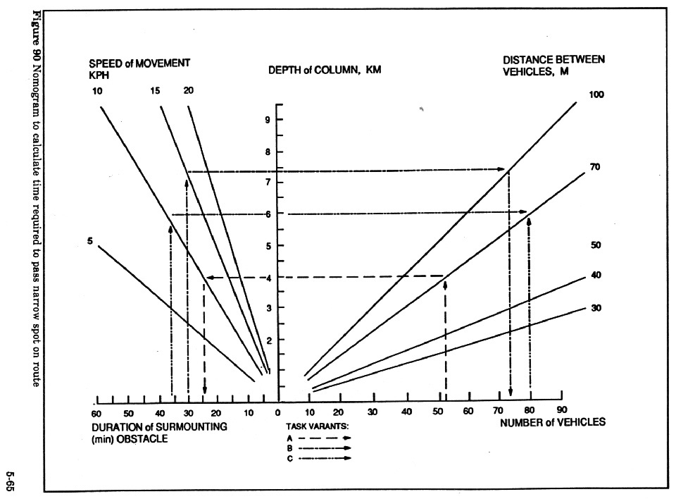
9 Calculation of Duration of Passage of Narrow Points and Difficult Segments

Example Calculation (A): Calculate the time required to cross an obstacle by a column of 54 vehicles with distance between vehicles of 75 meters and a maximum speed of 10 kph.

t=(54 x 75) x 0.06 ÷ 10=24 Min

There are two types of difficult sections on routes; the first is minor ones whose length is less than the marching column, and the second is major obstacles with length greater than the length of the column. The main factor for shorter obstacles is the number of vehicles in the column, the distances between them and their speed of movement while passing the obstacle. The main data for the larger obstacles are the length of the column, the length of the sector and the speed of movement.

The formula for major obstacles:

where:
G_k=length of column;
D=length negotiated segment;
t=duration to overcome obstacle in hours;
v=speed through obstacle.

Example calculation (B): Determine the time for a column 2.5 km long to pass through an obstacle 5.5 km long at a movement rate of 15 km per hr.

(2.5 + 5.5) ÷ 15=8 ÷ 15=0.53=32 min

Example calculation (C): Determine what length of column can negotiate a pass 2.5 km long at a speed of 8 kph in a 45 min. G_k=(V x t) - d=(8 x 0.75) - 2.5=3.5 Km

Solution: 3.5 km

Example using nomogram (Figure 90):

Example calculation: Using data from example (A), start at 54 on "Number of vehicles" line and draw a perpendicular to the intersection with the "Distances between vehicles - 74" line. From that point draw a horizontal line to the intersection with the "Travel speed - 10" line. From this point drop a perpendicular line to the "Duration of surmounting obstacle" scale at which point the result shows 24 minutes.

Example calculation variant B: Determine the number of vehicles able to cross an obstacle within 30 min, if the allowable movement speed is not more than 15 km per hr and the distance between vehicles is 100 m.

Solution: Start at 30 on "Duration of surmounting obstacle" scale, move vertically to "15 km per hr on speed" scale, then horizontally to "Distance between vehicles -100 m" and down to "Number of vehicles" scale where the result shows 75 vehicles.

Example calculation variant C: Calculate the distance between vehicles in a column of 80 vehicles in order that the column crosses a bridge within 36 min at rate not more than 10 kph.

Solution: Starting at 80 on the "Number of vehicles" scale and at 35 min on the "Duration of surmounting obstacle" scale draw perpendicular lines. From the intersection of the perpendicular with the "Speed of movement -10" scale draw a horizontal line to intersect with the first perpendicular. The point of intersection is on the "distance between vehicles- 75" line. This means that the distance between vehicles must be no more than 75 meters.

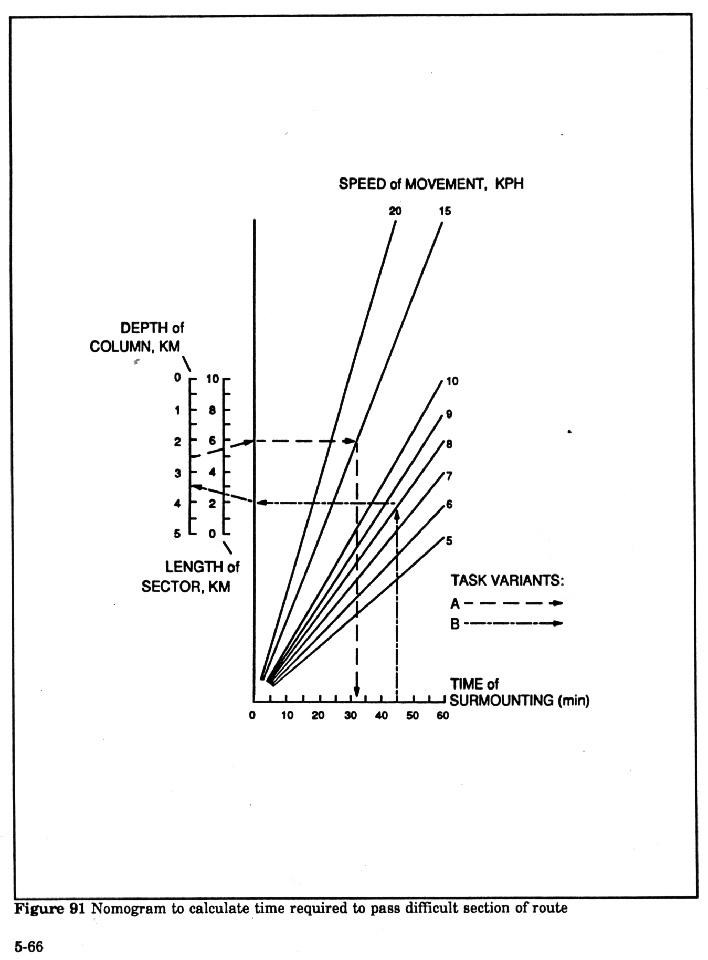Example using nomogram (Figure 91):

Example calculation variant A: Determine the time required to pass through a damaged strip of road, if the length of the sector is 5.5 km, the length of the column is 2.5 km, and the average speed while crossing the sector is 15 kph.

Solution: Mark on the "Depth of column" scale at 2.5 and the "Length of sector" scale at 5.5 and then draw a line through these points to the intersection with the Y or vertical axis. From this point draw a horizontal line to the "Speed of movement - 15" line and draw a perpendicular down to the "Time of surmounting" line to read the result of 32 min.


Example calculation variant B: Determine what length of column can negotiate a pass 2.5 km long at speed of 8 km per hr in a given time.

Solution: From the 45 mark on the "Time of surmounting" scale draw a perpendicular to the intersection with the "Speed of movement- 8" line. From this point draw a horizontal line to the Y axis. Connect this point with the 2.5 mark on the "Length of sector" line and continue it to intersect with the "Depth of column" line. This shows the result is 3.5 km. This means that a column of 3.5 km length may negotiate the passage in the given time.

Example Calculation (A): Calculate the time required to cross an obstacle by a column of ____ vehicles with distance between vehicles of ___ meters and a maximum speed of ____ kph.

t=(___ x ____) x 0.06 ÷ ___=___ Min


Example calculation (B): Determine the time for a column ____ km long to pass through an obstacle ___ km long at a movement rate of ____ km per hr.

(____ + ____) ÷ ___=__ ÷ ___=_____


Example calculation (C): Determine what length of column can negotiate a pass _____ km long at a speed of ____ kph in a ____ min. G_k=(V x t) - d=(8 x 0.75) - 2.5=3.5 Km

Solution: ____ km


Example using nomogram (Figure 90):

Example calculation: Using data from example (A), start at ____ on "Number of vehicles" line and draw a perpendicular to the intersection with the "Distances between vehicles - ___" line. From that point draw a horizontal line to the intersection with the "Travel speed - ___" line. From this point drop a perpendicular line to the "Duration of surmounting obstacle" scale at which point the result shows ___ minutes.

Example calculation: Determine the number of vehicles able to cross an obstacle within ____ min, if the allowable movement speed is not more than ____ km per hr and the distance between vehicles is ____ m.

Solution: Start at ___ on "Duration of surmounting obstacle" scale, move vertically to "____ km per hr on speed" scale, then horizontally to "Distance between vehicles -_____ m" and down to "Number of vehicles" scale where the result shows ____ vehicles.



Example calculation: Calculate the distance between vehicles in a column of ___ vehicles in order that the column crosses a bridge within ____ min at rate not more than ___ kph.

Solution: Starting at ___ on the "Number of vehicles" scale and at ____ min on the "Duration of surmounting obstacle" scale draw perpendicular lines. From the intersection of the perpendicular with the "Speed of movement -____" scale draw a horizontal line to intersect with the first perpendicular. The point of intersection is on the "Distance between vehicles- ____" line. This means that the distance between vehicles must be no more than ___ meters.


Example using nomogram (Figure 91):

Example calculation: Determine the time required to pass through a damaged strip of road, if the length of the sector is ____ km, the length of the column is ____ km, and the average speed while crossing the sector is ____ kph.

Solution: Mark on the "Depth of column" scale at ____ and the "Length of sector" scale at ____ and then draw a line through these points to the intersection with the Y or vertical axis. From this point draw a horizontal line to the "Speed of movement - ____" line and draw a perpendicular down to the "Time of surmounting" line to read the result of ___ min.


Example calculation: Determine what length of column can negotiate a pass ____ km long at speed of ___ km per hr in a given time.

Solution: From the ____ mark on the "Time of surmounting" scale draw a perpendicular to the intersection with the "Speed of movement- ___" line. From this point draw a horizontal line to the Y axis. Connect this point with the ____ mark on the "Length of sector" line and continue it to intersect with the "Depth of column" line. This shows the result is ____ km. This means that a column of ____ km length may negotiate the passage in the given time.

10 Calculation for Passage Times Across Start Point (SL) by the Head and Tail of the Column


Example: to determine the passage time of the starting line or other regulation point by the head and tail of the third column in a formation, when the passage time of the cited point by the tail of the previous column is 21:15, the established distance between the columns in 1.5 km, the depth of the column is 1.8 km and the movement speed is 25 km per hr.

solution:
t₃=21:15 + [(1.5) x (60)} ÷ 25=21:15 + 0.04=21:19;
t'₃=21:19=1.8 x 60 ÷ 25=21:19=0.04=21:23;

this means the third column in the march formation will pass the regulation point with its lead at 21:19 and its tail at 21:23 hrs.


Example calculation using the nomogram Figure 92: The nomogram may be used to speed up the calculation of the passage of a line by the head and tail of the column. To determine the passage time of an initial line by the head and tail of a march column 7 km line with the condition that the time for crossing the line by the tail of the lead column is 20:20, the distance between the columns is 5.5 km and the travel speed is 25 km per hr.

Solution: Draw a perpendicular line up from the horizontal axis, "Depth of column or distance between columns" scale from the 5.5 mark to the intersection with the "Average speed of columns -25" line. From this point draw horizontal line to the "Time of passing point" scale and read the result=13.3 or approximately 13 minutes. This is the time in which the head of the stated column must pass the point after it is passed by the previous column (at 20:00). The time for passing a point by the tail of a stated column is solved in a similar manner. For this draw a perpendicular line from the 7 mark on the "Depth of column axis" to the intersection with the "Average travel speed line - 25". From this point draw a horizontal line to the "Time of passing point" scale and read the result of 17 minutes. This means that this column must pass the control point with its tail at 20:30.



Example: to determine the passage time of the starting line or other regulation point by the head and tail of the _________ column in a formation, when the passage time of the cited point by the tail of the previous column is ______, the established distance between the columns in ____ km, the depth of the column is _____ km and the movement speed is ____ km per hr.

solution:
t₃=_____ + [(____) x (60)} ÷ ____=____ + _____=________;
t'₃=_________=_____ x 60 ÷ ____=_____=_____;

this means the _________ column in the march formation will pass the regulation point with its lead at ______ and its tail at ______ hrs.


Example calculation using the nomogram Figure 92: The nomogram may be used to speed up the calculation of the passage of a line by the head and tail of the column. To determine the passage time of an initial line by the head and tail of a march column ____ km line with the condition that the time for crossing the line by the tail of the lead column is ______, the distance between the columns is ____ km and the travel speed is ____ km per hr.

Solution: Draw a perpendicular line up from the horizontal axis, "Depth of column or distance between columns" scale from the _____ mark to the intersection with the "Average speed of columns -____" line. From this point draw horizontal line to the "Time of passing point" scale and read the result=____ or approximately ____ minutes. This is the time in which the head of the stated column must pass the point after it is passed by the previous column (at ______). The time for passing a point by the tail of a stated column is solved in a similar manner. For this draw a perpendicular line from the ___ mark on the "Depth of column axis" to the intersection with the "Average travel speed line - ___". From this point draw a horizontal line to the "Time of passing point" scale and read the result of ____ minutes. This means that this column must pass the control point with its tail at ______.

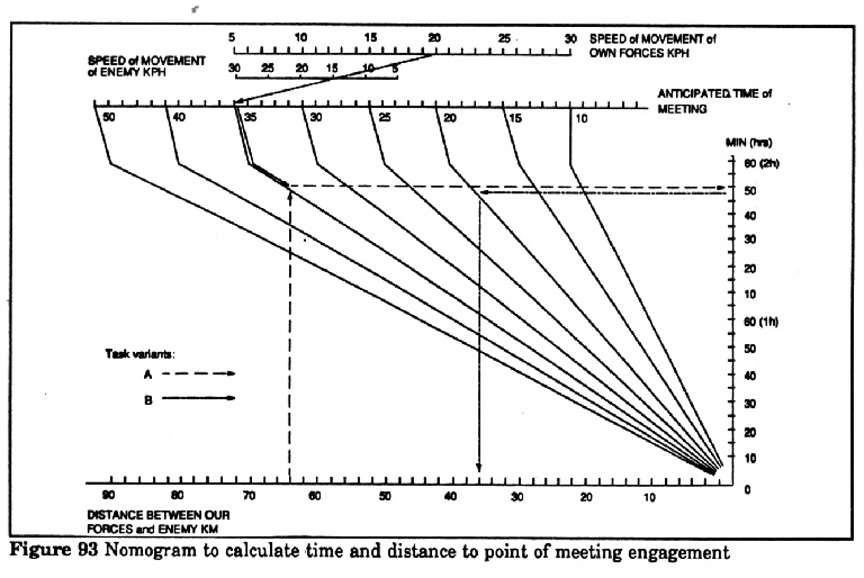
11 Calculation of Expected Time and Distance of Probable Point of Contact with Advancing Enemy


Example calculation: Determine the expected time of meeting and distance to probable encounter line when enemy is located 63 km away, his average forward speed is 25 km per hr, and average speed of friendly troops is 20 km per hr.

Solution: the equation yields distance of 28 km and time of 1 hr and 24 min.


Example using nomogram Figure 93: Determine the expected time of meeting and distance to line of contact with enemy if at 18:00 the advancing enemy is located at a distance of 64 km, his average speed is 15 km per hr, and friendly troops are moving at 20 km per hr.

To use nomogram (variant a) find the marks "20" and "15" on the "Speed of movement of own forces" and "Speed of movement of enemy" lines respectively, draw a line through these points to intersection with horizontal scale and read mark of 35. Then move downward along the line shown by the dots to the intersection with the perpendicular established from the "64" mark on the "Distance between our own and enemy forces" scale. From this point of intersection draw a horizontal line to the "Anticipated time of meeting" scale and read the calculation result of 1 hr and 50 min. This will be the length of time from the start time to meet the enemy. That means 18:00 plus 1:50 gives 19:50.

To determine the distance of the probable meeting line with the enemy (variant b) from the result of 1 hr 50 min, draw a horizontal line to the intersection with the speed line (ie at mark 20), which corresponds to the travel speed of the friendly troops. From the obtained point, drop a perpendicular line to the "Distance between friendly and enemy forces" scale and read the calculation result of 36 km.


Example calculation: Determine the expected time of meeting and distance to probable encounter line when enemy is located ____ km away, his average forward speed is ____ km per hr, and average speed of friendly troops is ____ km per hr.

Solution: the equation yields distance of ____ km and time of _______.


Example using nomogram Figure 93: Determine the expected time of meeting and distance to line of contact with enemy if at ____ the advancing enemy is located at a distance of ____ km, his average speed is ____ km per hr, and friendly troops are moving at ____ km per hr.

To use nomogram find the marks "____" and "___" on the "Speed of movement of own forces" and "Speed of movement of enemy" lines respectively, draw a line through these points to intersection with horizontal scale and read mark of ___. Then move downward along the line shown by the dots to the intersection with the perpendicular established from the "____" mark on the "Distance between our own and enemy forces" scale. From this point of intersection draw a horizontal line to the "Anticipated time of meeting" scale and read the calculation result of _____________. This will be the length of time from the start time to meet the enemy. That means _____ plus ____ gives _____.


To determine the distance of the probable meeting line with the enemy from the result______ draw a horizontal line to the intersection with the speed line (ie at mark ___), which corresponds to the travel speed of the friendly troops. From the obtained point, drop a perpendicular line to the "Distance between friendly and enemy forces" scale and read the calculation result of ____ km.

12 Calculation of Time Required for Advancing and Deploying Sub-units to Change From Line of March into the Attack


Determination of the time a unit should begin to move for the advance from its assembly area to the line of commitment into battle and assault on the enemy position is a complex application of the basic time and distance formula. All times are measured backwards from "CHE" hour, the moment the troops hit the first line of the defending enemy's position. The total time from beginning of movement in the assembly area is composed of the segments of time while moving in each type of deployment, that is: line of attack, company column, battalion column, and regimental column. It also includes the time it takes to shift from one formation to the other and any time for halts and delays en route. This is one of the most important and fundamental of tactical calculations. The times for sub-unit movement are tied exactly into the times for the artillery preparatory fire and air strikes.
The required given data are the distances between each of the deployment and regulating lines, distance of the attack line from the enemy's forward line of defense, distance of the start line from the unit assembly area, the average speed of movement while mounted in the columns, the coefficient for speed reduction during deployment actions, the speed of movement in attack formation, the depth of the columns, and distance between first and second echelons of the units.

To perform the calculation the required data may be entered into the table. The result will be the planning data for start of forward movement and deployment times for each shift of sub-unit columns. Since all times are measured backward from "Che", the planner must remember to subtract the values indicated in lines 12, 15, 18, 21, 24, and 27 from Che; and add the value for time in line 30 to the time in 24 to obtain line 31.

13 Calculation of the Time and Distance to the Line of Contact


Example problem: determine the expected time of meeting and the distance to likely line of contact with the enemy and the duration of movement to that line under following conditions:
----- start time of own forces - 20:00 hrs;
----- start time of enemy forces - 21:00 hrs;
----- distance to enemy - 105 km;

The commander decides there will be a break of 20 minutes (.3) hr during the advance. The plan is to delay enemy forces 30 -40 minutes (.6) hr. It is assumed that during movement enemy will be required to take halts of 30 minutes (0.5) hrs. The speed of movement of own forces is 28 km per hr. The speed of movement of the enemy is 19 km per hr.

The answer is that contact will be at 11:20 at a distance of 84 km. Duration of movement to meeting line is 3 hrs.


Example problem: determine the expected time of meeting and the distance to likely line of contact with the enemy and the duration of movement to that line under following conditions:
----- start time of own forces - _______ hrs;
----- start time of enemy forces - _______ hrs;
----- distance to enemy - ____ km;

The commander decides there will be a break of ____ minutes (____) hr during the advance. The plan is to delay enemy forces __________ minutes __ hr. It is assumed that during movement enemy will be required to take halts of _____ hrs. The speed of movement of own forces is ___ km per hr. The speed of movement of the enemy is ____ km per hr.

The answer is that contact will be at ____ at a distance of ___ km. Duration of movement to meeting line is ___ hrs.

14 Calculation of Expected Time and Rate of Overtaking when Pursuing the Enemy


Example: Determine how much time it will take for forces to overtake a retreating enemy when the distance to him is 20 km, his rate of retreat is 10 km per hr, and the rate of advance of friendly forces is 25 km per hr.

Solution: t_o=20 ÷ (25 - 10)=1.3 hrs ;


Determine the pursuit speed required to enable friendly forces to overtake enemy in 45 min, when he is 15 km away and his travel speed is 12 km per hr.

Solution: V_n=((15 + 0.75) (12)) ÷0.75=32 km per hr.


Examples of calculations using the nomogram Figure 96:


Determine the expected time to overtake enemy when his distance is 30 km, his travel speed is 20 km per hr, and the speed of pursuit is 28 km per hr. In the calculation (variant a) establish a perpendicular line from the "30" mark on the "Distance between friendly and enemy forces" scale. Then draw a line through the "28" mark on the "Friendly forces travel speed" and the "20" mark on the "Enemy travel speed" scale to its intersection with the horizontal upper axis. From this point draw a line down as shown by the dots to the intersection with the previously set perpendicular line. From the point of intersection draw a horizontal line to the right and read off the result of 3 hrs and 45 min on the "Expected encounter time" scale.

Determine the required pursuit speed to intercept the enemy in 1 hr and 20 min, when the enemy is at a distance of 40 km and is traveling at a speed of 5 km per hr.

In calculation (variant b) establish a perpendicular line from the "40" mark on the "Distance between friendly and enemy forces" scale to the intersection with the horizontal line, drawn from the 1 hr and 20 min mark on the "Expected encounter time" scale. From the meeting point draw a line, as shown by the dots and dashes, to the horizontal scale. Draw a line through the point of intersection of this scale and the 5 mark on the "Enemy travel speed" scale and continue it to the intersection with the "Friendly force travel speed" scale, where the result is 35 km per hr. This means that the pursuit speed must he at least 35 km per hr.


Example: Determine how much time it will take for forces to overtake a retreating enemy when the distance to him is ___ km, his rate of retreat is ___ km per hr, and the rate of advance of friendly forces is ___ km per hr.
Solution: t_o=___ ÷ (___ - ___)=____ hrs ;


Determine the pursuit speed required to enable friendly forces to overtake enemy in ____ min, when he is ___ km away and his travel speed is ___ km per hr.

Solution: V_n=((____ + ____) (___)) ÷ ____=___ km per hr.


Examples of calculations using the nomogram Figure 96:

Determine the expected time to overtake enemy when his distance is ____ km, his travel speed is ____ km per hr, and the speed of pursuit is ____ km per hr. In the calculation (variant a) establish a perpendicular line from the "___" mark on the "Distance between friendly and enemy forces" scale. Then draw a line through the "___" mark on the "Friendly forces travel speed" and the "___" mark on the "Enemy travel speed" scale to its intersection with the horizontal upper axis. From this point draw a line down as shown by the dots to the intersection with the previously set perpendicular line. From the point of intersection draw a horizontal line to the right and read off the result of _____ hrs on the "Expected encounter time" scale.

Determine the required pursuit speed to intercept the enemy in _______, when the enemy is at a distance of ___ km and is traveling at a speed of ___ km per hr.

In calculation establish a perpendicular line from the "___" mark on the "Distance between friendly and enemy forces" scale to the intersection with the horizontal line, drawn from the _____ mark on the "Expected encounter time" scale. From the meeting point draw a line, to the horizontal scale. Draw a line through the point of intersection of this scale and the ___ mark on the "Enemy travel speed" scale and continue it to the intersection with the "Friendly force travel speed" scale, where the result is ___ km per hr. This means that the pursuit speed must he at least ____ km per hr.

15 Calculation of the Work Time Available to the Commander and Staff for Organizing Repulse of Advancing Enemy Forces

Example: Determine how much time is available for the commander and staff to organize destruction of the advancing enemy if it is located at a distance of 25 km, his average speed is 15 km per hr, the effective range of the weapons is 12 km., and the time for preparing the sub-units is 30 min.

Solution: t={(25 - 12) x 60 ÷ 15} - 30=22 min.


Example calculation using the nomogram Figure 97: Determine the time the commander and staff spend in organizing the destruction of an advancing enemy if he is 15 km away, his rate of advance is 12 kph, the effective range of friendly weapons is 6 km, and the sub-unit preparation time is 20 min.

Solution: Mark the points "15" and "6" on the "Enemy distance" and "Effective range of friendly fire" scales, respectively. Draw a straight line through them to intersection with the vertical axis. From this point draw a horizontal line to the "Enemy advance speed - 12" line. From that point drop a perpendicular line to the horizontal axis and make a mark on it. Then draw a line through that mark to the "20" point on the "Time for preparing the sub-units for combat" scale. At the point of intersection of this line with the "Commander and staff work time" scale read the result of 25 min.


Example: Determine how much time is available for the commander and staff to organize destruction of the advancing enemy if it is located at a distance of ___ km, his average speed is ___ km per hr, the effective range of the weapons is ___ km., and the time for preparing the sub-units is ___ min.

Solution: t={(___ - ___) x 60 ÷ ___} - ___=___ min.


Example calculation using the nomogram Figure 97: Determine the time the commander and staff spend in organizing the destruction of an advancing enemy if he is ____ km away, his rate of advance is ____ kph, the effective range of friendly weapons is __ km, and the sub-unit preparation time is ___ min.

Solution: Mark the points "___" and "__" on the "Enemy distance" and "Effective range of friendly fire" scales, respectively. Draw a straight line through them to intersection with the vertical axis. From this point draw a horizontal line to the "Enemy advance speed - ___" line. From that point drop a perpendicular line to the horizontal axis and make a mark on it. Then draw a line through that mark to the "___" point on the "Time for preparing the sub-units for combat" scale. At the point of intersection of this line with the "Commander and staff work time" scale read the result of ____ min.

17 Determination of Quantity of Various Weapons, Reconnaissance, Support, Communications etc. for Task Performance


Example: Determine probability of spotting an enemy target with combined use of 3 reconnaissance systems, if their effectiveness expressed as the probability of detection of enemy target is:
P₁=0.4; P₂=0.6; and P₃=0.8

Solution:
P_n=1 - (1 - 0.4) x (1 - 0.6) x (1 - 0.8)=0.95 or approximately 1.


Example calculations using nomogram Figure 96: Determine the probability of enemy target destruction with a strike against it by three systems when the probability of target destruction by a single system of the particular type is 0.4.

Solution: (variant a) Draw a perpendicular from the "3" mark on the "Required number of systems" scale to the intersection with the "Probability of mission fulfillment by one system - 4" curve. From this point draw a horizontal line and on the "Probability of mission fulfillment by a group of systems" scale read that the probability of target destruction by three systems is 0.78.

It is possible to determine the reliability of communications in a link which consists of two channels (n=2), when the reliability of each channel is 0.6. From the nomogram, the probability of faultless operation of communications in this instance will be 0.84.

It is possible to evaluate the effectiveness of using four similar reconnaissance systems to detect an enemy target in an assigned region when the probability of detection by one system is 0.5. According to the nomogram, the probability of target detection by four systems will be close to one ).94.


Determine how many weapons systems must be assigned to inflict no less than 90% damage an enemy target, when the average damage inflicted byu a single system is 70%.

Solution: Draw a horizontal line from the "0.9" mark on the "Probability of mission fulfillment by a group of systems" scale to the intersection with the "Probability of mission fulfillment by a single system - 0.7" curve. From the intersection point drop a perpendicular line and on the "Required number of systems" scale find the result - 2. This means two systems must be used to achieve the assigned damage.


Example: Determine probability of spotting an enemy target with combined use of ___ reconnaissance systems, if their effectiveness expressed as the probability of detection of enemy target is:
P₁=____; P₂=____; and P₃=___

Solution:
P_n=1 - (1 - ____) x (1 - ____) x (1 - ____)=____.


Example calculations using nomogram Figure 96: Determine the probability of enemy target destruction with a strike against it by ____ systems when the probability of target destruction by a single system of the particular type is ____.

Solution: Draw a perpendicular from the "___" mark on the "Required number of systems" scale to the intersection with the "Probability of mission fulfillment by one system - ___" curve. From this point draw a horizontal line and on the "Probability of mission fulfillment by a group of systems" scale read that the probability of target destruction by three systems is ____.


Determine how many weapons systems must be assigned to inflict no less than ____ damage an enemy target, when the average damage inflicted byu a single system is ___.

Solution: Draw a horizontal line from the "____" mark on the "Probability of mission fulfillment by a group of systems" scale to the intersection with the "Probability of mission fulfillment by a single system - ____" curve. From the intersection point drop a perpendicular line and on the "Required number of systems" scale find the result - ___. This means ____ systems must be used to achieve the assigned damage.

19 Calculation of Strike Capability of Sub-units


Sample calculation: Determine the expected depth of penetration of attacking unit whose combat potential at 100% measures 150, during an attack on a enemy having a combat potential of 194 and a manning of 85%, if the attackers losses in the immediate battle reach 10% and the defender's losses reach 40%. The critical loss for the attacker is 50% and for the defender is 70%. The attack is conducted on a front of 5 km. The defending unit occupies an area of 8 km wide and 10 km deep, and the coefficient of effectiveness of the defender is 2.5.

This means the attacking unit can be expected to succeed in reaching a depth of 9.5 km in the defender's position. The Soviet author does not indicate the scale of this combat, and in fact uses the term for sub-unit (ie. a battalion or smaller), but from the dimensions of the combat area (8 km by 10 km) we may assume this is a regiment attacking of a brigade frontage to the full depth.

If we use the same formula to evaluate battle at division level we may assume "utils" of N_H=800 for attacker and N_O=700 for defender and the following other values for variables:
Y_N=90%; Y_O=80%; P_N=0.1%; P_O=0.4%; K=1.5;
P_N^K=0.5%; P_O^K=0.7%; F_O=20km; G_O=30km; F_N=15km;

The resulting equation is as follows:

With these assumptions the attackers may be expected to achieve a depth of penetration of 53 km.

Using the same formula to evaluate battalion scale combat we may assume both sides have "utils" of 40, the defender has a superiority coefficient of 2.5 and the widths are 4, 2, and 1.5 km. Then the formula yields the result as a penetration of 3.2 km. These are not unreasonable depths for the types of units being considered.

Sample calculation: Determine the expected depth of penetration of attacking unit whose combat potential at ___% measures ____, during an attack on a enemy having a combat potential of ____ and a manning of ___%, if the attackers losses in the immediate battle reach ____% and the defender's losses reach ____%. The critical loss for the attacker is ___% and for the defender is ____%. The attack is conducted on a front of ___ km. The defending unit occupies an area of ___ km wide and ___ km deep, and the coefficient of effectiveness of the defender is ____.

Solution:

Use the same formula to evaluate battle at division level we may assume "utils" of N_H=____ for attacker and N_O=____ for defender and the following other values for variables:
Y_N=____%; Y_O=___%; P_N=___%; P_O=___%; K=___;
P_N^K=____%; P_O^K=____%; F_O=___km; G_O=____km; F_N=___;

The resulting equation is as follows:

With these assumptions the attackers may be expected to achieve a depth of penetration of ____ km.

Using the same formula to evaluate battalion scale combat we may assume both sides have "utils" of ____, the defender has a superiority coefficient of ___ and the widths are __, ___, and ___ km. Then the formula yields the result as a penetration of ____ km. These are not unreasonable depths for the types of units being considered.

20 Calculation of the Width of Main Attack Sector


Example calculation: Given the width of full zone of action is 120 km, the overall correlation of forces is 1:1, the correlation of forces in the strike sector is to be 3:1, and the minimum allowable correlation of forces in the rest of the area is 0.5:1; determine the possible width of the strike sector.

Solution: W_m=120 (1 - 0.5) ÷ (3 - 0.5)=24 km.


Example calculation: Determine the correlation of forces possible in the strike sector given that the total width of zone is 400 km, the overall correlation of forces is 0.8:1, width of strike sector is desired to be 120 km, and the minimum correlation of forces allowable in the rest of the area is 0.5:1.

Solution: The formula may be restated as C_m=W_o ÷ W_m (C_o - C_s) + C_s ; inserting the given data produces a result of 1.5 as the possible correlation of forces for the strike sector. The commander may then decide on several alternatives such as narrow the strike sector, weaken the non-strike sector even more, bring in reinforcements, or weaken the defenders with preliminary artillery and air bombardments. Having done the initial calculation the commander may use the same formula in various ways while deciding on alternatives. For instance, to determine the required reenforcement to obtain a desired higher correlation the relationship is C=(1.25 - 0.8) ÷ 0.8 x 100=56.25%, that is by reinforcing by 56% the correlation in the overall area may be raised from 0.8 to 1.25 to 1.


Example calculation: Given the width of full zone of action is ____ km, the overall correlation of forces is ____, the correlation of forces in the strike sector is to be ___, and the minimum allowable correlation of forces in the rest of the area is _______; determine the possible width of the strike sector.

Solution: W_m=____ (1 - ___) ÷ (__ - ____)=____ km.


Example calculation: Determine the correlation of forces possible in the strike sector given that the total width of zone is ____ km, the overall correlation of forces is ______, width of strike sector is desired to be ____ km, and the minimum correlation of forces allowable in the rest of the area is _____.

Solution: The formula may be restated as C_m=W_o ÷ W_m (C_o - C_s) + C_s ; inserting the given data produces a result of ___ as the possible correlation of forces for the strike sector.

21 Calculation of Required Destruction of Enemy


Example calculation: In the break through sector regrouping of forces may bring the correlation of forces to 2:1, however for successful break through we need to bring the correlation up to 4:1 by means of initial artillery and air bombardment inflicting losses on the defenders. Determine what level of damage must be inflicted, if it is expected that the enemy will also inflict 30% loss on the attacking strike grouping.

Solution: M=100 - 2 ÷ 4 (100 - 30)=65%.


Assume that the initial "utils" of the attackers are 2000 and the defenders are 1000 for a correlation of 2:1. The enemy will inflict 30% losses bringing the attacking force to 1400 while the attackers must inflict 65% losses to bring the defender to 350 "utils" to achieve the 1400/350=4:1 ratio. For more rapid calculation of this relationship to determine the required losses to inflict one may use the following nomogram (Figure ). The nomogram is based on the above formula. The example shown is for the same situation. Enter with the correlation of forces 2 on the bottom left and draw vertical line to the correlation of forces 4 line, then a horizontal line across to the 30% loss line and again vertical down to read the required enemy loss of 65%.


Example calculation: In the break through sector regrouping of forces may bring the correlation of forces to ____, however for successful break through we need to bring the correlation up to ____ by means of initial artillery and air bombardment inflicting losses on the defenders. Determine what level of damage must be inflicted, if it is expected that the enemy will also inflict ____% loss on the attacking strike grouping.

Solution: M=100 - ___ ÷ ___ (100 - ___)=___%.


Assume that the initial "utils" of the attackers are ____ and the defenders are ____ for a correlation of ____. The enemy will inflict ___% losses bringing the attacking force to ____ while the attackers must inflict ___% losses to bring the defender to ___ "utils" to achieve the ____/____=__:___ ratio. For more rapid calculation of this relationship to determine the required losses to inflict one may use the following nomogram (Figure ). The nomogram is based on the above formula. The example shown is for the same situation. Enter with the correlation of forces ___ on the bottom left and draw vertical line to the correlation of forces ___ line, then a horizontal line across to the ___% loss line and again vertical down to read the required enemy loss of ____%.

22 Calculation of Rate of Advance in Relation to Correlation of Forces


Example calculation: A given strike group has a planned average rate of advance of 40 km per day. Determine what the required correlation of forces superiority is to achieve this rate.

Solution: Taking the formula V ÷ 140=K_C or 40 ÷ 140=0.29. Enter 0.29 on the scale for K_C in the nomogram and draw a horizontal line to the curve and then a vertical line down to the scale of correlation of forces scale. This shows a required correlation of about 3.4:1 for the strike sector.


Example calculation: In the zone of action of the strike group we have created a 2.5:1 superiority in correlation of forces. Determine the approximate tempo of advance.

Solution: From the nomogram read that the correlation of 2.5:1 corresponds to a K factor of 0.13. Then using the formula V=140 x 0.13=18.2 km per day advance rate.


Another approach is to use the following formula to calculate a factor corresponding to the K factor in the previous method. In the following nomogram the rate of advance is related also to movement distance, terrain type, length of the operation and a theoretical maximum movement speed. These variables are joined into a single factor according to the equation: F=D ÷ KTV_max where:
D=distance (depth) of operation;
K=terrain coefficient (1.25 - level; 1.00 - rough-level; .75 - rugged hills; .75 - urban; .50 - mtns.)
T=time required for operation in days and fractions of days;
V_max=theoretical speed in km per day.


According to this nomogram, to achieve a depth of advance of 30 km on level terrain in one day with a theoretical maximum speed of 60 km per day requires a superiority in correlation of forces of 4:1. With a correlation of forces of 3:1 on rough-level terrain and a theoretical maximum speed of 50 km per day in two days the force may advance 20 km.


Example calculation: A given strike group has a planned average rate of advance of ___ km per day. Determine what the required correlation of forces superiority is to achieve this rate.

Solution: Taking the formula V ÷ 140=K_C or ___ ÷ 140=____. Enter ____ on the scale for K_C in the nomogram and draw a horizontal line to the curve and then a vertical line down to the scale of correlation of forces scale. This shows a required correlation of about ___:__ for the strike sector.


Example calculation: In the zone of action of the strike group we have created a ___:__ superiority in correlation of forces. Determine the approximate tempo of advance.

Solution: From the nomogram read that the correlation of ___:___ corresponds to a K factor of ____. Then using the formula V=140 x ____=____ km per day advance rate.


Another approach is to use the following formula to calculate a factor corresponding to the K factor in the previous method. In the following nomogram the rate of advance is related also to movement distance, terrain type, length of the operation and a theoretical maximum movement speed. These variables are joined into a single factor according to the equation: F=D ÷ KTV_max where:
D=distance (depth) of operation;
K=terrain coefficient (1.25 - level; 1.00 - rough-level; .75 - rugged hills; .75 - urban; .50 - mtns.)
T=time required for operation in days and fractions of days;
V_max=theoretical speed in km per day.

According to this nomogram, to achieve a depth of advance of 30 km on level terrain in one day with a theoretical maximum speed of 60 km per day requires a superiority in correlation of forces of 4:1. With a correlation of forces of 3:1 on rough-level terrain and a theoretical maximum speed of 50 km per day in two days the force may advance 20 km.

24 Determine the Required Amount of Manpower and Weapons for Bringing Sub-Units back up to Sufficient Strength to Restore their Combat Capability

Example calculation using the table: Determine the required number of tanks and guns to re-equip a sub-unit if the required level of superiority is 2.5:1, the initial full strength of own troops was 85% (0.85), the losses of own forces in tanks is 40% (0.4), the initial full strength of the enemy was 60% (0.6), his losses in tanks are 40% (0.4).

Solution: Entering the data in the table we find that to resupply the sub-unit and restore its combat capability requires 2 tanks. Replacements of guns are not required since, given the losses on both sides, the required level of superiority necessary to fulfill the mission is preserved.


Example calculation using the table: Determine the required number of tanks and guns to re-equip a sub-unit if the required level of superiority is ____:1, the initial full strength of own troops was ___% (____), the losses of own forces in tanks is ___%, the initial full strength of the enemy was ___%, his losses in tanks are ___%.

Solution: Entering the data in the table we find that to resupply the sub-unit and restore its combat capability requires __ tanks. Replacements of guns are not required since, given the losses on both sides, the required level of superiority necessary to fulfill the mission is preserved.

25 Determine the Expected Radiation Dose


Example calculation using the form: Determine the possible radiation doses of personnel of a subunit while they are negotiating two zones of radioactive contamination with mean radiation levels of 187 and 165 roentgens per hour. The length of the route within the first zone is 12 km and the second is 10 km. The travel speed of the sub-unit is 25 and 18 km per hr respectively. The first zone is crossed along a route perpendicular to the pattern axis and the second at an angle to the pattern axis. The reduction coefficient is 4.

Solution: performing the calculations using the table we find that the total radiation dose received by personnel may reach 15 roentgens.


Example calculation using the form: Determine the possible radiation doses of personnel of a subunit while they are negotiating ____ zones of radioactive contamination with mean radiation levels of ____ and ___ roentgens per hour. The length of the route within the first zone is ___ km and the second is ___ km. The travel speed of the sub-unit is ___ and ___ km per hr respectively. The first zone is crossed along a route perpendicular to the pattern axis and the second at an angle to the pattern axis. The reduction coefficient is ___.

Solution: performing the calculations using the table we find that the total radiation dose received by personnel may reach ___ roentgens.

 

29 Calculation to Determine the Effectiveness of Fire Destruction Means

Example problem: Determine the expected number of destroyed targets from 30 observed targets, if 12 weapons with a rate of fire of 3 rounds a minute are used for their destruction. The probability of destruction by 1 shot is 0.2 and firing time is 5 min. The probability of destruction of our weapon by enemy in the time of one shot is .3

Example problem: Determine the expected number of destroyed targets from ___ observed targets, if ___ weapons with a rate of fire of ___ rounds a minute are used for their destruction. The probability of destruction by 1 shot is ___ and firing time is ___ min. The probability of destruction of our weapon by enemy in the time of one shot is ___