| |
Figure 63 - Aerial Reconnaissance
|
|
| |
AERIAL RECONNAISSANCE
UNITS IN THE FRONT AIR ARMY
|
| UNIT |
NUMBER AIRCRAFT |
DEPTH OPERATION |
| Operational Recon Regt |
30 bomber type |
800 - 1000 km |
| Tactical Recon Regt |
40 fighter type |
400 - 500 km |
| Combat Regiments |
10 - 12 outfitted for recon
also |
|
|
| |
An air army, which has five divisions and three
reconnaissance aviation regiments, can have 287 reconnaissance aircraft and 377
pilots, including 60 tactical reconnaissance aircraft and 30 operational
reconnaissance aircraft. Fifteen percent of the non-organic reconnaissance
aviation is designated for carrying out reconnaissance. In this case the
reconnaissance aviation on the first day will carry out 500-700 flights.
Reconnaissance crews in an area of 10-15 kilometers can reconnoiter 2-3 targets
in one flight.
In the front there are 3-4 tactical pilotless aviation squadrons. Each
squadron has 4 aviation flights. The squadron can conduct in all 36 pilotless
reconnaissance sorties. Each squadron is attached for reconnaissance in support
of a first echelon army. The time of flight is 45 minutes, the width of
photography is 5 kilometers, the overall range of photography is 75 kilometers.
The squadron can conduct reconnaissance as follows:
|
|
| |
Figure 64 - Drone reconnaissance aircraft
|
|
| |
Drone reconnaissance
aircraft
|
| Flight altitude |
Flight Radius |
| 600 meters |
80-100 km |
| 3000 meters |
150-170 km |
| 7000 meters |
200- 250 km |
|
|
| |
Space Reconnaissance
The Soviet Union uses space reconnaissance means at a distance of 200-250
kilometers above the earth. A single pass can photograph a 40-50 kilometer
zone.
|
|
| |
Figure 65 - Visual Reconnaissance Range
|
|
| |
VISUAL
RECONNAISSANCE RANGES FROM AIRCRAFT
|
| Limits of Range of
Detection and Distinguishing Objects (Targets) Daylight in Good
Visibility |
| Object |
Flight Altitude |
Slant Range, km Detection |
Distinguish |
| Artillery in fire positions,
uncamouflaged |
100 |
2-3 |
1.-1.5 |
| 300 |
3-3.5 |
2-3 |
| 600 |
3-4 |
2-3 |
| 1000 |
3-4 |
2-3 |
| 4000 |
5 |
undistinguish-able |
| Rocket launcher, artillery
guns, automobiles, tanks, armored transporters, radar stations on the ground
and in movement in columns along highways and on dirt roads,
uncamouflaged |
100 |
4-5 |
2-3 |
| 300 |
6-7 |
3-4 |
| 600 |
6-7 |
3-4 |
| 1000 |
6-9 |
4-5 |
| 6-7000 |
10-12 |
Undistinguish-able |
| 8-10,000 |
12-15 |
" |
| Tanks, automobiles, armored
transporters under cover in trenches, camouflaged |
100 |
3-4 |
1.5-2 |
| 300 |
6-7 |
3-4 |
| 600 |
6-7 |
3-4 |
| 1000 |
6-7 |
4-5 |
| 4000 |
7-8 |
5 |
| Tanks, automobiles, armored
transporters, uncamouflaged |
4-500 |
3-4 |
1-2 |
| 2-3000 |
4-5 |
- |
| 3-4000 |
5-6 |
- |
| Artillery and mortar
trenches, camouflaged against terrain background |
4-5000 |
5-6 |
Undistinguish-able |
| 5-6000 |
8-10 |
" |
|
|
| |
Artillery Reconnaissance
An army artillery reconnaissance regiment has 2 battalions: the first battalion
has a sound ranging battery (zvukovaia razvedka), one radio-technical
reconnaissance battery, and one optical reconnaissance battery; the second
battalion has a photography battery, a topo-geodetic battery, and a
meteorological service battery.
|
|
| |
Figure 66 Artillery
Reconnaissance
ARTILLERY
RECONNAISSANCE EXPECTED LOCATION ERRORS
|
| Reconnaissance System |
Range Error - % Range from
Observer |
Deflection Error - % Rg from Observer or
m |
| Visual Recon Theodolite |
0.5-0.8 |
0.1 |
| Stereoscopic Telescope |
0.8-1.1 |
0.2 |
| Range finder |
1.0-1.5 |
0.2-0.3 |
| (Dependent on range finder base) |
(1.0-1.2) |
(0.1) |
| Flash ranging |
Large (0.5-0.8) |
Large (0.1) |
| Timing flashes |
Large |
- |
| Sound Ranging |
1.0 (1.0) |
0.4 (0.4) |
| Helicopter Recon |
(1.4) |
(0.9) |
| Radar |
A few meters |
| Visual Detection from an Aircraft (No
instruments) |
100-150 meters CEP (50-70
meters) |
| Aerial Photo |
15-20 meters CEP |
|
|
| |
Air Defense Reconnaissance
An army PVO radio-technical battalion can conduct reconnaissance to a depth of
80-100 kilometers on a front of 160 kilometers (at great heights and average
heights) and on a front of 80 kilometers, (at low and very low heights). An
army PVO radio-technical battalion has 4 companies. The battalion is deployed
in two echelons. In the first echelon are two companies at a distance of 10
kilometers from the forward edge. The distance between the two companies is 50
kilometers. On the width of the army zone, two companies are situated in the
first echelon, and two companies are in reserve to build up the radar posts in
the course of the offensive. The radio-technical battalion will relocate once
in 24-36 hours at a distance of 30-50 kilometers during the operation.
|
|
| |
Electronic Reconnaissance
The radio and radio-technical company of a division has 3 platoons of
interception and radio direction. The company can establish 5 interception
posts, 3 direction finding posts, 3 radio-technical posts.
- depth of radio reconnaissance 25-30 km; Radio-technical - 60 km;
- radio interception numbers 3-4 radio nets;
- radio direction net of 2-3 posts; 30 verified fixes an hour;
- RT can take a bearing of an average of 20-30 radar stations per hour and can
determine their technical specifications;
- SNAR - 2 ground targets up to 16 km; water targets up to 38 km;
- sound ranging battery deploys 4-6 km; covers 6-8 km, depth of reconnaissance
18 km.;
- flash spotting battery deploys 5 km covers 6-8 km, depth of recon 12-15 km;
- reconnaissance detachment (Co) 4-5 km sector, Div 30-40 km; Regt 20-25 km;
- recon group of 4-5 platoons;
- RCP 6-8 km from Bn.
A separate radio battalion (osnaz) at army level has the following:
- 3 radio intercept companies - 23 posts;
- 1 radio direction finder company - 10 posts;
- 1 reconnaissance helicopter flight.
A separate radio-technical battalion (osnaz) has the following;
- 3 radio-technical companies - 24 radio-technical and 11 radio intercept
posts;
- 1 reconnaissance helicopter.
The battalion can carry out reconnaissance on ground targets to a depth of up
to 60-120 kilometers and reconnaissance on aerial to a depth of 300-350
kilometers.
A separate front radio regiment (osnaz) has the following;
- 2 radio intercept battalions;
- 5 radio direction finder companies;
- 1 radio relay reconnaissance company;
- 1 reconnaissance helicopter;
- 1 laboratory.
The regiment can set up 125 posts, including 97 radio intercept and 28 radio
direction finder posts. Radio direction finder posts can conduct reconnaissance
at a depth of 1000 kilometers with a width of 500 kilometers. The radio
interceptor post can conduct reconnaissance to a depth up to 2000 kilometers.
A separate front radio-technical regiment has the following:
- 2 radio-technical battalions;
- 1 radio interceptor battalion
- 1 aviation reconnaissance flight;
- 1 laboratory.
The regiment can organize 97 posts, including 46 radio-technical and 50 radio
interceptor posts. The aviation reconnaissance has 2 airplanes, which have
radio-technical means. The regiment can conduct reconnaissance at a depth of
500-2000 kilometers.
During the organization of the first offensive operation, the radar means of
the army do not operate, but the reconnaissance of the enemy is conducted with
front equipment. Two to four radar posts of the front will be
located in the army zone.
The second echelon of radar is organized by forces of the front. It is
situated 50 kilometers from the forward edge.
|
|
| |
Planning for Reconnaissance
Soviet combat doctrine places a strong emphasis on extensive reconnaissance.
Soviet planners consider detailed knowledge of the defender's unit locations
(front line strong-points, reserve assembly areas, artillery positions, and
command posts) to be essential. They expect to have such information available
in timely fashion.
To obtain this information the Soviet commander is served by an extensive
reconnaissance establishment that includes agent networks, SPETZNAZ units, and
long range reconnaissance units under army, front, and TVD control;
air reconnaissance from front and TVD; combat patrols from divisions;
radio and radio-electronic combat units at army and front; artillery
sound ranging and counter battery target acquisition units; engineer and
chemical warfare reconnaissance units from divisions, army, and front;
and national technical intelligence collection platforms which provide reports
through front intelligence headquarters.
The commander of an army or front in the Western TVD, for instance,
has a priceless intelligence file containing information built up over 40 years
on every nook and cranny in his operating area. One might speculate that the
potential volume of information available to the Soviet commander is so massive
that the principle limitation on its effective exploitation is his own finite
human ability to master it.
The Soviet planner expects to have the information needed to serve his purposes
available when he wants it. He organizes the collection effort and flow of
information through the analysis process accordingly.
The following is the phased sequence of information flow related to the
decision /planing process. This shows that the level of detail required in the
information increases as the planning process moves from general outline of the
concept to specific targeting of force on force. It shows that the Soviet norm
for timeliness allows more time for the acquisition of the more detailed
information.
|
|
| |
Information for the Estimate of the
Situation
This information is required within 2-3 hours of the start of planning:
- grouping, disposition, and nuclear weapons;
- movement and likely intentions;
- strength and composition;
- weak points in dispositions;
- meteorological situation.
For the Commander's Decision
The following information is required within 4-6 hours of start of planning:
- changes in disposition;
- nuclear delivery means;
- density of troops and means in one km of front;
- density on each axes and along the entire front;
- disposition down to regiment or brigade level;
- location of artillery;
- exact location of command posts;
- support aircraft locations
For Detailed Planning
The following information is required within 12-24 hrs of start of planning:
- exact location of battalions on the ground;
- exact location of support arms;
- location of mine fields;
- location of nuclear delivery means and artillery bns;
- location of reserves and logistic support elements;
- fortifications;
- air defenses and anti-tank weapons systems locations;
- airfield composition and support aircraft.
The time to prepare the reconnaissance report of the chief of reconnaissance
for his commander is shown in this table.
|
|
| |
Figure 67 Preparation time for
Reconnaissance
TIME REQUIRED TO
PREPARE RECONNAISSANCE REPORT
|
| for regiment commander |
15-20 min. |
| for division commander |
30-60 min |
| for army commander |
1-1.5 hr |
| for front commander |
2-3 hr |
| for commander TVD |
4-5 hr |
|
|
| |
Norms in Planning Air Army Operations
The average time to prepare the air army daily plan of operation is 2-3 hrs.
During battle, to launch a squadron of fighters or fighter bombers requires 10
min. and a regiment requires 20 min., if the unit is in category 1 readiness.
In an air operation, when bomber and fighter-bomber aviation strike against
enemy airfields, 20-30% of fighter aviation will escort and cover them during
the action.
During a front offensive operation, the main effort of the
front aviation is concentrated at a depth of 30-40 kilometers from the
front line and sometimes up to 80 kilometers.
During actions to support a front offensive operation, the aviation
can operate initially with a capability of 3-4 sorties per day tapering to
1.5-2 sorties toward the end of the operation. The movement of one aviation
squadron from one airfield to another deployment airfield will take 30-60
minutes (including take-off, travel time, landing, and replenishment).
A fighter-bomber and a fighter regiment each consists of 43 planes. If the
division has in its composition 3 regiments of each, this division will have in
its composition 130 fighter-bombers and 130 fighters.
Only one aviation regiment is located on one airfield. If the conditions are
good, one regiment can be deployed at two airfields. A squadron is located at a
distance far from other squadrons, so that one medium nuclear blast will not
destroy two squadrons. The distance between planes is 200 meters. A caponier
(an earth parapet made of dirt piles around the current position) is built
around each aircraft to protect it from fragments of enemy bombs.
At readiness # 1 for fighter aviation and fighter-bomber aviation units: the
crew is located in the airplanes, and with the reception of a signal, the
aviation regiment becomes airborne in 8-10 minutes. At readiness #2 for fighter
aviation and fighter bomber aviation units: the crew is located near the
airplanes, and with the reception of a signal, the regiment becomes airborne in
about 20 minutes.
|
|
| |
Figure 68 Tactical Technical Characteristrics of
Transport Aircraft
BASIC
TACTICAL-TECHNICAL CHARACTERISTICS OF TRANSPORT AIRCRAFT
|
| Main Features |
AN-12 |
AN-22 |
| Crew |
7 |
7 |
| Maximum speed (km/hr) |
683 |
710 |
| Average speed |
500 |
-- |
| Flight Altitude (meters) |
12000 |
11000 |
| Weight in Air: Minimum |
54 |
196.5 |
| Maximum |
61 |
225.0 |
| Maximum range (km) |
6450 |
8800 |
| Load Capacity: Maximum |
20 |
-- |
| Normal |
10.6 |
50 |
| Passenger Capacity: Troops |
93 |
295 |
| Paratroops |
60 |
152 |
| Wounded |
80 |
177 |
| Tactical Radius (km) |
900 |
-- |
|
|
| |
Planning Factors for Airborne Operations
The depth of an air drop or an air landing depends on its scale and type as
follows:
- a strategic operational desant - 500-600 kilometers;
- an operational desant in conventional war - 150-300 kilometers;
- an operational desant in nuclear war - 300-400 kilometers;
- an operational-tactical desant in conventional means is 100-150
kilometers;
- an operational-tactical desant in nuclear war - 250-300 kilometers;
- a tactical desant - 50-100 kilometers or more.
An airborne division can continue its operation independently for 6-7 days. The
division is dropped at a distance so that, after 2-3 days, the main forces
reach the area of the division landing. This distance will be 150-300
kilometers from the front line.
A transport aviation regiment consists of 32 airplanes. If the division has 4
regiments, then the division will have 130 planes. A transport aviation
division of four regiments can make an air landing or air drop of one parachute
regiment. A parachute regiment of 1600 people will its weigh 700-800 tons. For
the landing of one desant division by means of parachutes, 455 AN-12
planes are required, broken down as follows: for the transport of the parachute
dropping group 415 planes are needed, and for the landing group 40 planes are
needed. For a parachute regiment to be dropped 80 AN-12 airplanes are needed,
or one transport aviation division.
A transport aviation regiment of the type AN-12 can become airborne in the
following times according to readiness status:
- readiness #1 in 15 minutes;
- readiness #2 in 1 hour;
- readiness #3 in 4 hours.
According to the experience of exercises bringing the military transport
aviation from routine combat readiness to full combat readiness requires 25-27
hours. Included in this, to raise by an alarm requires 2 hours; to prepare the
troop control of transport aviation )organization of airborne operations(
requires 81 hours. For loading the airplanes and completing the preparation of
military transport aviation, 2-3 hours are required.
If military transport aviation received the mission beforehand, and it is
located at the permanent or deployment airfields in the first or second degree
of readiness for take-off, the time for preparation significantly decreases, in
this case the time will be 5-7 or 5-8 hours.
One airborne )desant( division is air dropped on one flight in 4-5
hours; by landing )air landing( method, the process requires 20-28 hours.
For each military transport division composed of 3-4 regiments, 4 main
airfields and 1-2 reserve airfields are needed. Up to 20 airfields are needed
to deploy 4 military transport divisions in the staging area; included in this,
16 of the airfields will be main airfields and 4-6 will be reserve airfields.
The same number of airfields are designated for strategic aviation,
front aviation, and front and national air defense and civil
aviation.
For resupply of one AN-12 aircraft, 3- 15 tons of fuel are needed. At one
airfield, at which one transport regiment is concentrated, up to 500 tons of
fuel are required. At all 20 airfields, for 4 transport divisions, from
10,000-12,000 tons of fuel are needed. The assembly area/waiting area of an
airborne division is designated at a distance of 5-10 kilometers from the
airfield. The area of the staging area for an airborne division can be 300 by
400 kilometers.
Fuel resupply areas for military transport aviation are designated at a
distance of 200-300 kilometers from the front.
The time for landing, fuel resupply, and take-off of one military transport
regiment will be 2-3 hours. The flight of aviation to the desant area,
the boarding of the desant on the aircraft, fuel resupply and take-off
of aviation from the staging area to the objective of the air drop requires 7-9
hours. To load military equipment requires 2-3 hours, and it must be finished
30-50 minutes before the take-off. At the same time the fuel resupply is being
carried out and the military transport regiment is brought up to readiness #2.
The boarding of personnel is concluded 10-15 minutes before starting the
engines of the aircraft and the regiment is brought to combat readiness #1. The
boarding of personnel requires 10- 20 minutes. The speed of the flight of
transport aviation is 500 km/hour.
The depth of the formation of a transport regiment during flight will be 32
kilometers during the day and 110 kilometers at night. The time of the air drop
of one regiment during the day will be 4 minutes, and at night it will be 13
minutes. The depth of a military transport division formation during flight
will be 180 kilometers during the day and up to 900 kilometers at night.
The time of the air drop of one division will be 25 minutes during the day and
1 hour 47 minutes at night.
An airborne division can carry with it material reserves for two full days.
Each day an airborne division expends in their combat activities 250 tons of
material. To supply such a load of material, 20-25 AN-12s are required.
Air transport of the troops in great distances is more advantageous, because at
a distance of 500 kilometers, the average speed of movement is 50 km/hour; at a
distance of 3000 kilometers, the average speed of movement will be 215 km/hour;
at a distance of 6000 kilometers, the average velocity of movement will be 250
km/hour. The conditions of the above calculations are the following: transport
and movement of troops, two hours are needed; for loading, 4 hours are needed;
for unloading, 3 hours are required. The average speed of the flight is 500
km/hr.
The requirement of military transport aviation for transport of a motorized
rifle division without heavy equipment is 803 AN-12s; the transport of a
motorized rifle regiment without heavy equipment requires 138 AN-12s; the
transport of an artillery regiment requires 122 AN-12s.
For the supply of one basic ammunition load and one refueling of POL for a
motorized rifle regiment, 30 AN-12s, or almost one transport regiment, is
needed.
|
|
| |
Norms in Air Defense Planning
The time to assemble a battalion, move, deploy, and take a new position depends
on distance, with 10 min to assemble and 20-30 min to deploy. A regiment takes
15 min to assemble. The time to move varies with the distance. At the new
location it requires 30-40 min to deploy and be ready to fire.
Capability:
The front air defense is capable of destroying 15-25 percent of the
enemy aviation, which participates in a massive strike. Losses of PVO in the
enemy first nuclear strike will be 20-35 percent, but with the use of only
conventional weapons the losses will be 5-10 percent.
Location:
The depth of the air defense belts in a strategic operation will be:
- First Echelon Second Echelon 300-500 kilometers. 700-1000 km
The SA-2 rocket regiments of an army and front are located at a
distance of 10-20 kilometers from the FEBA. The distance between battalions is
10-30 kilometers. The regimental command point is located in the center where
its distance should not be more than 20 kilometers from the battalions. The
technical battalion deploys in the rear of the rocket regiment. The distance to
the furthest rocket battalion should not exceed 30 kilometers. The distance
between rocket battalions should not be less than 5 kilometers, so that one
nuclear blast will not destroy two battalions.
In crossing a wide water obstacle )rivers(, the position of the forward air
defense rocket battalions will be as follows:
- SA-2 rocket battalions - 10-11 kilometers from the bank of the river;
-SA-3 rocket battalions - 6 kilometers from the bank.
Composition:
Front
Forces and means of the air defense of a front which has in its
composition 3 combined arms and one tank army and one air army will be the
following )without consideration of the division PVO forces and means(:
- 6-11 anti-air rockets of the type SA-2
- 1-2 PVO divisions;
- 4-8 separate antiaircraft artillery regiments of the type S-60;
- 1-2 anti-air rocket regiments of the type SA-3;
- 1 PVO radio-technical regiment;
- 4 PVO radio-technical battalions;
- 2-3 fighter aviation divisions including 6-9 regiments.
The front - level PVO forces and means are the following:
- 2-3 PVO rocket regiments of the type SA-2;
- 1-2 PVO rocket regiments of the type SA-3;
- 1 antiaircraft artillery division;
- 1 radio-technical regiment.
Army
The organic air defense means and forces of the army are the following:
- 1-2 PVO rocket regiments of the type SA-2;
- 1-2 antiaircraft rocket regiments of the type S-60;
- 1 radio-technical battalion.
|
|
| |
Air Defense Army
The composition of an army of the national PVO is not constant. It depends on
the mission, importance, direction, and nature of the theater, and on the
number of targets which are being defended. The PVO army, which has in its
composition 1-2 corps and 2-4 PVO divisions, will have the following forces and
means:
- 5-7 PVO rocket brigades;
- 15-20 PVO rocket regiments;
- 6-12 fighter aviation regiments;
- 3-6 radio-technical regiments or brigades;
- 1 separate radio-technical regiment of spetsnaz;
- 2-3 separate radio battalions of spetsnaz;
- 1 signal center and engineer, chemical, rear services and other units
In a continental theater of military operations )TVD( the following PVO forces
and means participate:
- 100-150 formations and units of rocket troops;
- 30-40 fighter aviation regiments;
- 50-70 antiaircraft artillery units;
- 30-40 radio-technical formations and units;
- 3-4 radar patrol boats;
- 60-80 air defense artillery ships.
Radio-technical means of the front conduct the reconnaissance of the
enemy at a depth of 300 kilometers at great and average heights and at a depth
of 150 kilometers and also at very low heights, along a width of 120
kilometers. The command post of the PVO of a front simultaneously
reports 40-45 targets, while the command post of the PVO of an army reports 30
targets.
|
|
| |
Factors Used in Calculating Air Defense
Capabilities
There are several types of factors, weapons effective numbers for individual
weapons, and expressions of general capability associated with SAM and air
defense artillery units. Air defense has been one of the most dramatically
improving branches of the Soviet armed forces during the past 15 years. Thus
the technical characteristics and associated capabilities factors for air
defense weapons and radar systems are continually changing. The following
factors were official as of the mid-1970's and may be taken as characteristic
examples of the type of factors used in Soviet planning methods. However, for
assessments of current capabilities they should be significantly increased.
According to the experience of Soviet exercises the attrition on Soviet forces
from the enemy first massive air strike may be:
- in nuclear conflict: 20-35%
- in conventional conflict: 5-l0%
|
|
| |
Destruction Coefficients of Selected
SAM Weapons
| WEAPONS |
WITH JAMMING |
WITHOUT JAMMING |
| S-75M (SA-2( |
0.45-0.72 |
0.66-0.77 |
| S-125 )SA-3( |
0.4 |
0.7 |
| STRELA-2M )SA-7( |
0.22-0.26 |
0.72-0.76 |
|
|
| |
Fire Capabilities of Selected Units
- S-75 )SA-2( regiment can engage one target at a time and shift after two
minutes
- S-60 AAA regiment of division can engage one target at a time ) 24 guns(
- S-60 AAA regiment of army can engage two targets at a time ) 36 guns(
- infantry and tank regiment air defense battery can engage one target at a
time and shift after one minute
- STRELA-2M squad )three launchers( can engage one target at a time with
destruction probability 0.53-0.60:
- formula used to convert the weapons effectiveness of individual weapons into
that for a unit or group of weapons is as follows: P=1 - )1 - P(n
- using the effectiveness of the individual Strella to compute the
effectiveness of the squad gives the indicated value. P=1 - )1 - 0.22( )1 -
0.22( )1 - 0.22(=0.53
The formula is generally used to determine how many weapons are required in
order to reach a certain desired effectiveness. Thus P is given and the
equation is solved for n. A table giving the values for P achieved by each n
can also be constructed.
|
|
| |
Rear Service Norms and Planning Factors
The following information on the organization and capabilities of army and
front level rear service organizations has been taken from the
lectures delivered at the Soviet General Staff Academy in the mid-1970's.
Army Rear Services:
The army material support brigade )MSB( can maintain up to 7,000 tons of
material. It can have up to 7,000 men and 2,500 transport vehicles. The army
MSB has as its components the following units, subunits, and establishments:
- base headquarters;
- signal platoon;
- separate chemical defense company;
- separate rear services signal battalion;
- separate gas decontamination battalion.
A state bank branch is one of the components of a rear mobile army base branch,
as is a mobile bakery plant )with a capacity of 18 tons in a 24 hour period(
and a military post office, a military shopping )trade( facility with a
capacity of 40 tons, personnel of all types of supply )artillery, armor, motor,
engineering, chemical, signal, POL, foodstuffs, clothing, medical, furniture(
and a service company, which can load or unload 2500 tons in a 24 hour period.
The Army MSB has various supply storage facilities )depots(. The capacity of
each is as follows:
- artillery depot - 2000 tons;
- fuel depot - 3000 cubic meters;
- food depot - 400 tons;
- tank depot - 1000 tons;
- motor tractor depot - 150 tons;
- engineer depot -250 tons;
- signal depot - 80 tons;
- chemical depot - 300 tons;
- goods and property depot - 40 tons;
- medical depot - 60 tons;
- quarters depot - 25 tons;
- trade depot - 40 tons.
A motor transportation regiment in the brigade has 4 battalions and one
battalion for transporting POL. The regiment can transport up to 5,000 tons,
including 630 tons of POL.
Two separate road construction and traffic battalions are designated for
preparing the army's main vehicle roads. These battalions are not part of the
mobile support brigade.
The rear services of an army are also composed of the following rear units:
- separate battalion for the recovery of tanks;
- separate company for the recovery of motor transport equipment;
- separate engineer company for recovery and repair.
An army can receive from the front several rear services units and
establishments, such as a tank repair battalion, and a separate automobile
repair battalion.
The air army also has as one of its components a rear service. In the rear
service of an air army there are the following units and establishments:
- the rear services headquarters;
- 1-2 air army mobile bases;
- one separate technical support regiment )each division has aviation technical
support battalions; each regiment also has technical support battalions(;
- separate companies for technical support of the airfields.
In the staging position for an offensive, the army material support brigade and
rocket technical base are located 40-60 kilometers from the front, and reserve
positions are 15- 20 kilometers from the main locations. If several formations
of an army operate on separate axes, a branch of army's material support
brigade is designated to resupply and reinforce them. The rear units and
establishments move forward in accordance with the rate of advance. As a rule,
the medical support detachment, motor ambulance company, and units for recovery
and repair of damaged vehicles move behind the first echelon divisions.
An army material support brigade is located so that its distance will not be
more than 125 kilometers, i.e., one half of the daily march, from the division
material support battalions. At a rate of advance of 30-50 kilometers per 24
hour period, the army material support brigade relocates once every 2-3 days.
The rocket technical base, as a rule, moves behind the units of rocket troops.
Some of the rear services of the army, such as the army mobile base, army
rocket technical base, mobile mechanical bakery, separate recovery and repair
battalion for armored vehicles, and recovery company for motor transport,
relocate in one move, while other elements shift locations in increments.
The organization of the rear services in a defensive operation:
In an offensive, the depth of the rear services of a division will be up to 40
kilometers, and in defense, the depth of the rear services of a division will
be up to 60 kilometers. Division medical battalion, separate medical
detachments which the division has received as reinforcement, and the repair
battalion, are located between the first and second echelons of the division,
or in the depth of the division defense. The remaining units of the division
are situated at a distance of 30-40 kilometers from the FEBA, behind the combat
formation of the division. The rear of second echelon divisions of the army,
and the rear of other, which are located in the units, as a rule, are located
in the region of the deployment of such divisions and units. The depth of the
army rear services area in defense will be 100-150 kilometers.
The rear services of an army is deployed as follows:
- the army rocket technical base is at a distance of 30-40 kilometers from the
positions of the army rocket troops, or 60-80 kilometers from the positions of
the rocket battalions of the divisions;
- the army material support brigade is situated at a depth of 100-120
kilometers from the forward edge, or 60-80 kilometers from the divisions'
material support battalions;
- a branch army material support brigade on a separate direction is situated at
a distance of 60-80 kilometers from FEBA;
- the separate recovery and repair battalion for tanks, and a the separate
recovery and repair company for motor transport vehicles, and the ambulance
company are situated behind the first echelon divisions for the recovery of
equipment and vehicles, and the sick and wounded;
- the separate medical detachments which are in the reserve of the army are
situated behind the second echelon divisions near the rear command post of the
army.
Their relocation to alternate positions is conducted, in accordance with the
order of from the chief of the rear services of the army, in case of threat to
their position or use of chemical weapons.
|
|
| |
Technical support of the army:
During World War II, 8-9 percent of the tanks were knocked out of operation
every twenty four hours. With the use of nuclear weapons, these losses will be
12-15 percent every 24 hours. The technical repair means of the troops can
handle 100% of the running light repair and 15-20 % of the medium repair.
During a nuclear war, in the course of an operation losses will be as follows:
50-80%; 30-40 percent of the APCs; 40-50 percent of wheeled vehicles.
|
|
| |
Front Rear
Services:
The composition of the rear services of a front is not constant; it
depends on the composition of the front, the mission, and the
conditions of the theater of military operations. The rear services of the
front are made up of 250-300 rear services units and installations,
consisting of 160,000-170,000 men, up to 25,000-27,000 vehicles. The following
rear services formations, units and installations make up the rear of a
front:
- 1-2 rear service bases of the front;
- 2-3 forward bases of the front;
- 4-6 forward hospital bases of the front;
- 2-3 hospital bases of the front;
- 2-3 automobile transportation brigades )each brigade can load 6600 tons,
including 1440 tons of POL(;
- 2-3 railroad brigades (each brigade can lay 20-25 kilometers of railroad in a
24 hour period, or up to 9 kilometers of railroad when it has been completely
destroyed);
- 2-3 road construction and commandant service brigades )each brigade can
reconstruct up to 900 kilometers of road; it can reconstruct a bridge with a
load capacity of 60 tons, length of 110 kilometers(, can establish 16 traffic
regulation posts, can construct a 400 meter floating bridge of 16 tons;
- 2-3 pipeline brigades )each brigade can put together 600 kilometers of
pipeline; in a 24 hour period the brigade can refuel, using pipe with a
diameter of 100 millimeters, 800 tons of fuel, and with pipe with a 150
millimeter diameter, 2000 tons of fuel over a length of 75-150 kilometers. In a
24 hour period, it can lay 65-75 kilometers of pipe(;
- separate battalions for transport of rocket fuel )each battalion can
transport 640 tons of rocket fuel(;
- rocket fuel depots of the front )each depot can store 500 cubic
meters of rocket fuel(;
- separate medical ambulance battalions )in one trip each can evacuate up to
0003 sick and wounded(;
- separate air transport medical regiments )including 23 AN-2 airplanes; in one
flight a regiment can evacuate 180 seriously ill men(.
A front has the following units and installations for recovery and
repair, which are subordinate to the chiefs of services: ) 17 repair plants and
evacuation units(:
- separate railroad exploitation regiments;
- separate rear services signal regiments of the front;
- guard division for the protection of the rear services;
- bridge construction brigade, )it is a central reserve and establishes
crossing sites on wide rivers(;
- railroad bridge construction brigade.
The following is the organization of some of the rear installations: As a rule
the front mobile base is designated to resupply armies of the first
echelon with material requirements. Its capacity is 8000 tons of materials.
Which meets 3-4 day requirements of the respective grouping of forces to be
resupplied. A front forward base is assigned to one or two armies. In
its composition are the following elements: base headquarters, storage
facilities )each type of supply has 1 control element(. The capacity of each
facility is as follows:
- artillery depot - 250 wagon loads 38 cubic feet per load(;
- fuel depot - 4000 cubic meters;
- food depot - up to 250 wagon loads;
- tank depot - 250 wagons;
- motor and tractor depot - 25 wagons;
- engineer troop depot -200 wagons;
- communications depot - up to 70 wagons;
- chemical depot - up to 150 wagons;
- light goods and property depot - up to 150 wagons;
- medical depot - 300-350 wagons;
- topographic depot - up to 500 wagons.
A front forward base also has as part of its composition the
following:
- 2 separate service companies )each company can load or unload up to 2500
tons(;
- an engineer company;
- a separate chemical defense company;
- 3 mobile field bakeries;
- repair plants for repair of equipment organic to POL, food, and clothing
services;
- lubricant reprocessing station;
- two field mobile laundry detachments;
- laboratory;
- military post office;
- automobile transport regiment with a load capacity of 3300 tons.
The headquarters of the base includes a chief of the base, his deputy,
political assistant, planning and organization section, movement section, six
assistant chiefs for supply of ammunition and armament, POL, motor-tractor,
tank, food-clothing, and combat technical equipment. The front rear
base can maintain material reserves for 10 days. As a rule it is situated on a
railroad. The load capacity is 57,000 tons. The organizational structure is as
follows: base headquarters depots with capacities as follows:
- artillery depot - 250 wagons;
- artillery weapons - 250 wagons;
- POL depot - 8000 cubic meters;
- food depot - up to 350 wagons;
- tank depot - up to 250 wagons;
- motor tractor depot - up to 150 wagons;
- engineer depot - up to 200 wagons;
- signal depot -up to 100 wagons;
- goods and clothing depot - up to 150 wagons;
- chemical depot - 500 wagons;
- medical depot - up to 800 tons;
- veterinary depot - up to 7 wagons;
- household goods depot - up to 50 tons.
Besides this, the front rear base has in its composition a separate
transport battalion with a load capacity of 1100 tons, a separate engineer
company, a separate service battalion (the battalion can load and unload 7500
tons in a 24 hour period(; a separate chemical defense company, 3 mechanical
field bakeries and other repair and other units including, repair plants to
repair equipment used by POL, food and clothing, supply services, two mobile
POL reprocessing stations, 7 field laundry detachments, centers for unloading
and distribution of front transportation, testing laboratory, field
post office. The composition of the rear base headquarters is the same as
forward base headquarters.
The deployment and relocation of the rear services of the front:
The boundaries of the front rear service area are determined by the
rear services directive from the supreme commander-in-chief. In the FUP area it
is located up to 400 kilometers from the forward edge. As the leading divisions
in the offensive move forward, the depth of its location increases and may
reach 1000 kilometers. The rear services deploys in two echelons. In the first
echelon are the following elements: the forward base of the front is
located behind the armies of the first echelon at a distance of 80-100
kilometers, near the railroads in an area of 150 square kilometers; rocket
technical units, which are located at a distance of 30-40 kilometers from the
positions of the rocket troops; rocket fuel depots and pipeline units and large
units; the forward hospital base of the front, which is located 50-70
kilometers from the FEBA; recovery and repair units of the front, as a
rule, are located in the area of the armies or are given to the armies as
reinforcement. The second echelon is situated in the following manner: the rear
base of the front is situated on a railroad; it is deployed in a large
area. The zone covers an area of 200 kilometers wide by 50-100 kilometers in
depth. Storage facilities are located along the railroad in the depth. As a
rule the rear hospital base of a front is situated in 2-3 regions by a
railroad. Its distance from the forward edge will be 50-70 kilometers, or
200-300 kilometers. When there is a railroad, its distance will be the greater
one, i.e. 200-300 kilometers.
Repair plants are situated, as a rule, near the front rear bases, and
use local plants if possible. If the front has two rear bases, each
base will be situated on separate axes to resupply the armies. One branch of
the rear base of a front is located at 120-150 kilometers from the
FEBA; and the second branch remains in the reserve to be used during the
operation.
Relocation of the front rear during an offensive operation:
The first echelon of the front rear services should not fall behind
the armies rear services more than 150 kilometers, i.e., not more than one half
of the length of supply movement over a 24 hour period. If the speed of the
offensive is 45-50 kilometers per 24 hour period, the first echelon will be
relocated once in three days. If the speed of the offensive is 80-100
kilometers, the first echelon will be relocated once every two days.
The front forward base, as a rule, relocates at full strength. If
conditions require, it can send forward a branch.
The mobile rocket technical base of the front relocates behind the
advancing troops each time after 150-200 kilometers, or they relocate once
after 220-250 kilometers, so that their distance will not be more than 340
kilometers from the positions of the rocket troops. Rocket fuel depots
simultaneously relocate with the rocket technical bases.
Mobile repair units of the front approach the sectors where a large
number of damaged combat equipment is massed, and conduct repair work.
Formations, units, and installations of the second echelon of the rear services
of a front move forward with the preparation of the railroad. The
front rear base, in the course of an offensive operation, sends
forward, in turns, its branch. It relocates in full strength only at the end of
an operation.
Organization of supply of material in the offensive operation of the
front: The principle of resupply is from above downward. Resupply is
carried out continually with the use of the sum total of all types of
transport. Under conditions of using nuclear weapons, the volume of overall
resupply of a front will be 300,000 tons; with the use of conventional
weapons, the overall volume of resupply of the front will be 450,000
tons, in which one third of the resupply will be the air army, PVO troops,
various reserves, and the rear services of the front. Resupply of the
first echelon armies will be 20,000 tons per 24 hour period.
The average daily (24-hour) haul of transport means of a front will be
300 kilometers; for transport means of an army this will be 250 kilometers; for
troop transport, this will be 200 kilometers.
|
|
| |
Some Fundamentals of Troop Supply:
Material reserves are replenished up to the norms every day. The first priority
for delivery of resupply is those troops which are successful in the operation.
All types of transport )front, army, troops( are used together.
Front second echelon troops organize resupply by means of their own
transport. As a rule, when the troops are moving forward very fast or an
airborne assault is being air landed, resupply and transport is organized by
air, and airfields are prepared. Superfluous loading is prohibited, that is,
loading from one vehicle to another; this wastes time. It is better when the
materials and ammunition are resupplied on one vehicle, for example, from a
front depot and unloaded at a division depot.
The role of the types of transport:
Resupply from the front forward base to the army material support
brigade amounts to 90% by motor transport means and 5% by air transport means.
From the front rear base to the front forward base, 15% of
the transport is by railroad, 70% is by motor transport means, 10% is by
pipeline, and 5% is by air transport. To the front rear base, 75 % of
the transport is by rail, 15 % is by motor transport, and 10% is by pipeline.
The preparation, content, and use of roads for a front offensive
operation: as a rule, in an offensive operation all types of transport routes
are used, such as railroad, waterways, air lanes, vehicular roads, and
pipelines. In the area of the front there will be 2-3 front
railroads and 2-3 lateral railroads. Their capacity will be 70 pairs of trains
in a 24 hour period. In the course of the operation, 1-2 railroad axes are
prepared with a capacity of 30 pairs or trains in a 24 hour period. 40-45
kilometers of rail can be laid by two railroad brigades in a 24 hour period;
under conditions of mass destruction, 20-25 kilometers can be laid in this
period. As a rule, for an army 2-3 distribution stations and 1-2 reserve
stations are allocated.
Unloading stations are allocated to an army as follows: one per division, 2-3
for the army material support brigade. One or two temporary loading areas are
organized for a front.
Waterways: A distribution port is designated for a front; an unloading
port is designated for an army.
Front military vehicular roads:
These roads join the front bases with their branches, and with the
army mobile bases. Behind each first echelon army of the front there
is one frontal military vehicular road. The capacity of this road will
be up to 01,000 vehicles in a 24 hour period.
Main field pipeline:
It is designated for the transport of fuel from the permanent and
front storage facilities )depot( to the troops. As a rule, it is laid
in the direction of the main attack of the front.
Military air transport:
- 7-8 percent of the material resupply is carried out by military air
transport.
Requirements/expenditures on an Operation and Creation of Reserves at the end
of the Operation
The material requirements at the front will be up to 700,000 tons.
Included in this will be the following:
- small arms ammunition: 4-4.5 basic loads;
- artillery and mortar ammunition: 7.5-9 basic loads;
- tank ammunition: 7.5-9 basic loads;
- antiaircraft ammunition: 8.5-9.5 basic loads;
- aviation ammunition: 22-32 basic loads;
- motor gasoline: 8-9 refuelings;
- diesel: 11-31 refuelings;
- aviation gasoline: 26-27 refuelings;
- food: 30 daily rations.
|
|
| |
Figure 69 - Echeloning Reserve Material of the
Front
ECHELONING
RESERVE MATERIAL AT THE FRONT
|
| Ammunition )basic load |
Fuel
Refueling |
Food daily rations
|
|
Small Arms |
Arty & Mortars |
Tanks |
Anti Air |
Aviation |
Gas |
Diesel |
|
| Troops |
1.0 |
1.0 |
2.25 |
2.0 |
|
1.7 |
2.4 |
13 |
| Army )2 days( |
0.15 |
0.3 |
0.4 |
0.5 |
|
0.46 |
0.7 |
2 |
| Air army reserves |
1.75 |
|
|
|
17.5 |
3.0 |
3.5 |
21 |
| Forward base of the front |
0.22 |
0.45 |
0.6 |
0.7 |
|
0.6 |
1.0 |
3-4 |
| Rear base of the front |
0.78 |
1.5 |
2.0 |
2.55 |
|
0.3 |
3.5 |
01 |
| Total |
2.15 |
3.25 |
5.25 |
5.75 |
17.5 |
5.15 |
7.65 |
28-29 |
|
|
| |
Figure 70 - Norms for Material Reserves in an
army
NORMS OF RESERVE MATERIAL AND ITS ECHELONING DURING
WAR
|
| Ammunition )basic Loads( |
Fuel )refueling( |
Food )daily ration( |
|
Small arms |
Arty and mortars |
Rockets |
Tanks |
Antiair |
Gas |
Diesel |
|
| Army storage |
0.15 |
0.3 |
0.3 |
0.4 |
0.5 |
0.46 |
0.7 |
2 |
| Troops storage |
1.0 |
1.0 |
1.0 |
2.25 |
2.0 |
1.7 |
2.4 |
13 |
| Division storage |
0.2 |
0.2 |
0.2 |
0.75 |
0.5 |
0.4 |
0.75 |
2 |
| Units |
0.8 |
0.8 |
0.8 |
1.5 |
1.5 |
1.3 |
1.65 |
11 |
| Total 6-7 days |
1.15 |
1.3 |
1.3 |
2.65 |
2.5 |
2.16 |
3.1 |
15 |
|
|
| |
Figure 71 - Requirements for material reserves in
Offensive
ARMY MATERIAL REQUIREMENT IN A OFFENSIVE OPERATION
|
| Ammunition (basic load) |
Fuel (refueling) |
Food daily ration |
|
Small arms |
Arty and mortars |
Tanks |
Antiair |
Gas |
Diesel |
| Use in operation(nuclear) |
1.0-1.6 |
2.1-3.2 |
2.4-3.2 |
3.5-5.6 |
1.4-2.4 |
2.8-4.0 |
7-8 |
| Use in operation (non-nuclear) |
|
|
|
3.5-5.6 |
1.4-2.4 |
2.8-4.0 |
7-8 |
| Creating reserves toward the end of the
operation |
1.15 |
1.3 |
2.65 |
2.5 |
2.15 |
3.1 |
15 |
| Overall need on an operation )nuclear( |
2.15-2.75 |
3.4-4.5 |
5.5-5.85 |
6.0-8.6 |
3.56-4.56 |
5.9-7.1 |
22-23 |
| Overall need on an operation
)non-nuclear( |
|
|
|
6.0-8.6 |
3.56-4.56 |
5.9-7.1 |
22-23 |
|
|
| |
Figure 72 - Operational Expenditure and
Reserves
OPERATIONAL EXPENDITURE AND RESERVES
|
| Echelons |
Ammunition (basic loads) |
Fuel (refueling) |
Food )daily rations( |
|
Infantry weapons |
Arty and mortar |
Tank |
Air defense |
Air |
Auto fuel |
Diesel |
Aviation fuel |
| Total in front |
2.15 |
3.25 |
5.25 |
5.75 |
17.5 |
5.15 |
7.65 |
15.0 |
28-29 |
| Troops |
1.0 |
1.0 |
2.52 |
2.0 |
-- |
1.7 |
2.4 |
-- |
13 |
| Army (2 days) |
0.51 |
0.3 |
0.4 |
0.5 |
-- |
0.64 |
0.7 |
-- |
2 |
| Air army |
1.57 |
-- |
-- |
-- |
17.5 |
3.0 |
3.5 |
7.5 |
21 |
| Forward rear base |
0.22 |
0.45 |
0.6 |
0.7 |
-- |
0.6 |
1.0 |
-- |
3-4 |
| Front rear base |
0.78 |
1.5 |
2.0- |
2.55 |
-- |
2.3 |
3.5 |
7.5 |
10 |
| Total require- ment |
4-4.5 |
7.5-9 |
7.5-8 |
8.5-9.5 |
22-32 |
8-9 |
11-31 |
26-27 |
30 |
|
|
| |
Figure 73 - Location of Rear Supply and
Support
LOCATION OF REAR SUPPLY AND SUPPORT
ELEMENTS
|
| 1st Echelon sub-units/units |
Approximate depth from battle
zone |
| Offensive Defensive |
| COMPANY: First aid post |
--- |
50-100 m |
| Ammo distribution points |
--- |
100-150 m |
| Rations & water point |
--- |
up to 1 km |
| BATTALION: Medical post |
1-2 km |
1.5-3 km |
| Ammo distribution points |
3 km |
2-3 km |
| Rations and field kitchen |
3 km |
2-4 km |
| Technical observation post |
1-2 km |
2-4 km |
| REGIMENT: Medical post |
5-7 km |
6-10km |
| Transport platoon |
5-7km |
up to 20km |
| POL point |
10-15km |
10-20km |
| Ammo Distribution points |
10-15km |
10-20km |
| Rations |
10-15km |
10-20km |
| TK & MT repair & evacuation group |
up to 8km |
up on 10km |
| Damaged vehicle collection pound |
5-7km |
6-10km |
| 2nd echelon regiments - All rear service elements |
16-20km |
|
| DIVISION: Medical post |
10-14km |
up to 20km |
| Truck repair & depot |
10-14km |
up to 20km |
| Tank repair & depot |
20-40km |
35-60km |
| Arty & small arms repair/depot |
20-40km |
35-60km |
| Transport Bn |
20-30km |
20-40km |
| Engineer Bn |
20-40km |
35-60km |
| Ammo dump |
25-30km |
35-50km |
| POL dump |
25-30km |
35-50km |
| Rations dump & field bakery |
25-30km |
35-50km |
| Baths/laundry/water |
25-30km |
40-45km |
| 2nd echelon divisions - All depots |
40-70km |
|
|
|
| |
Medical Norms and Planning Factors
Army medical support:
The following medical units are components of the rear services of an army:
- 10-12 separate medical detachments in a combined arms army )OMO(;
- 6 separate medical detachments in a tank army )OMO(;
- a separate ambulance company )ASR(;
- a separate anti-epidemic medical detachment )ASPEO(;
- an army medical reinforcement detachment )OMU(;
- a veterinary-epizootic detachment )VEO(.
Each medical battalion of a division and separate medical detachment can take
in a 24 hour period up to 500 men. The evacuation capability of a medical
battalion of a division is 80 sick and wounded per trip; a separate medical
detachment can evacuate 160 men on one trip; the medical ambulance company of
the army can evacuate up to 1000 sick and wounded per trip.
The army medical anti-epidemic detachment and reserve medical detachment, and
army medical reinforcement detachment are located between the first and second
echelon of the army near the army command post. Separate medical detachments
and recovery and repair subunits, which are attached to reinforce first echelon
divisions operate in the division zone.
Front medical support:
There are up to six forward hospital bases in the front. The capacity
of each base is 6500 beds. Each base has 13 separate hospitals, such as a
mobile surgical unit, mobile therapeutic unit, and a mobile neuropathological
unit, as well as others. There are also various sub-units, units, and
installations. A front has 2-3 rear hospital bases. The overall
capacity of a rear hospital base of a front is 20,000 beds, including
5900 beds in mobile hospitals and 14,100 beds in evacuation hospitals. The base
is situated in 2-3 regions near the railroad. It has 48 various
hospitals/units, including a medical ambulance company, a special medical
support battalion, and others. The forward hospital bases of the front
are deployed near the centers of large personnel losses, usually about 40-50
kilometers from the front line.
|
|
| |
Casualty estimates
During World War II losses of personnel were 0.8-1.0 percent in a 24 hour
period. With the use of nuclear weapons, this loss of personnel would be
3.70-5.30 percent per day. In all operation there will be 27-42 percent losses.
With the use of conventional weapons, losses will be 1.10-1.30 percent in a 24
hour period, while in the entire operation this will be 7.40-01.40 percent.
At the front level with the use of nuclear weapons, losses of
personnel for the entire operation will be 35-40%; in a 24 hour period losses
will be 2-2.06%. In accordance with the type of weapons, losses will be as
follows:
- nuclear weapons - 16-18 %;
- conventional weapons )artillery fire, rifle, and aviation( - 6-7 %;
- chemical weapons - 5-6%;
- biological weapons - 1.5-2%;
- disease - 1.5-2%.
The greatest losses will be during the first nuclear strike: losses will be up
to 33% of all losses. With the use of conventional weapons, losses for the
entire operation will be 12-13%; on the average, in a 24 hour period losses
will be 0.7-0.9%. With respect to the above mentioned losses, 120,000-130,000
hospital beds, including 40,000-50,000 at the beginning of the operation will
be needed. The fact that a front does not have such a quantity of beds
means that 2 men will have to be put on one bed to provide for the treatment of
the sick and wounded )each bed is multiplied by two(.
The following are the allowable doses of radiation from nuclear blasts for
personnel:
- once in the course of every four days - up to 50 roentgens;
- several times in the course of 10-30 days - 100 roentgens;
- several times in the course of 3 months - up to 200 roentgens;
- several times in the course of one year - 300 roentgens.
The contamination from nuclear blasts is measured and affected areas are
divided into zones. The outermost zone ) A ( varies from 40 to 400 roentgens,
the next, ) B( is from 400 to 1200, the next )C( is from 1200 to 4000, and the
innermost zone )D( is from 4000 to 10000:
- the average zone of destruction )zone A(: contamination doses on an external
border - 40 roentgens, and on an internal border - 400 roentgens;
- the zone of strong contamination )zone B(: on an external border - 400
roentgens, and on an internal border - 1200 roentgens;
- the a zone of dangerous contamination )zone C(: for an external border - 1200
roentgens, and for an internal border - 4000 roentgens;
- the zone of extremely dangerous contamination )zone D(: for an external
border - 4000 roentgens, and for an internal border - 10,000 roentgens.
|
|
| |
Protection against nuclear radiation
The most effective means for reducing the destructive action of penetrating
radiation are various types of coverings. The cover may be layers of iron,
concrete, brick, or earth, as well as combat equipment found in sub-units.
The protection effectiveness of a material used for a cover depends on the
density and thickness of the layer. Heavy materials such as lead, steel,
concrete, and ferro-concrete have the greatest absorption capability, and,
thus, the greatest capability for reducing gamma radiation. Walls of concrete
or brick protect to a greater degree than wooden ones or ones built of foamed
concrete. Dirt has good protection properties and, practically speaking, the
greatest value as a covering material. This is illustrated by data included in
the table.
The use of coverings as protection against neutrons is a very complex problem.
Materials with high density, which are good protection against gamma radiation,
do not provide sufficient protection against neutrons. And it should be
remembered that emission of secondary gamma radiation accompanies the capture
of neutrons by the nuclei of the atoms. In this respect it is necessary to use
materials which weaken gamma radiation. Materials used as protection against
neutrons can be divided into three groups:
- the first is materials which slow down fast neutrons;
- the second is materials which absorb neutrons which have been slowed down;
- the third is materials which weaken secondary gamma radiation.
Light materials containing much hydrogen )paraffin, water, some plastics( are
used to slow neutrons down, and materials such as cadmium, boron, and others
are used to absorb neutrons. Some of the above-mentioned materials are employed
as elements of anti-neutron finishes used in new generations of combat
vehicles.
Concrete and moist earth are also good protection against neutrons and gamma
radiation. Although they do not contain elements with a high atomic mass, they
do, however, have a sufficiently high amount of hydrogen so as to slow down and
capture neutrons, and a sufficient amount of limestone and silicon so as to
absorb gamma radiation. In connection with this, a sufficiently thick layer of
concrete or moist earth can be used to assure simultaneous protection against
neutrons and gamma radiation.
The factors for reducing the penetrating radiation of a neutron explosion by
combat vehicles are, respectively:
- armored personnel carrier - 1.1-1.2
- BMP - 1.5
- tanks without an anti-neutron cover - 1.5-2.0
- tanks with anti-neutron cover - as much as 10 times.
In protection activities field fortification installations can be used for
protection against penetrating radiation. The multiplying factor of reducing
the dosage of the penetrating radiation from atomic, fission, thermonuclear,
and neutron explosions is given in the table.
|
|
| |
Figure 74 - Protection against
radiation
Layers for Partial
Reduction )in centimeters( of Penetrating Radiation for Several Protection
Materials
|
| Type of material |
Density of material kg per
cu decimeter |
Radiation |
| Gamma |
Neutron |
| Fission |
Synthesis |
Fission |
Synthesis |
| Armor |
7.8 |
3.5 |
3.5 |
11.0 |
12.0 |
| Concrete |
2.3 |
9.5 |
12.5 |
8.2 |
9.8 |
| Brick wall |
1.6 |
13.0 |
18.0 |
9.0 |
11.0 |
| Earth |
1.6 |
13.0 |
18.0 |
9.0 |
11.0 |
| Water |
1.0 |
20.4 |
28.0 |
2.7 |
4.9 |
| Polyethylene |
0.9 |
21.8 |
31.0 |
2.7 |
4.9 |
| Wood |
0.7 |
30.5 |
40.0 |
9.7 |
14.0 |
|
|
| |
(A layer for partial reduction is a layer of material which
reduces by half the strength of the dosage of radiation)
|
|
| |
Figure 75 - Coefficients of
reduction of Radiation
Coefficients of
Reduction of the Total Dosage of Penetrating Radiation From a Nuclear Explosion
by Field Fortification Objects
|
| Type of object |
Protection layer )in
centimeters( |
Type of
explosion |
| Surface |
Air |
| Atomic charge: q >/=10
thousand tons |
| Field Shelter |
140 |
600 |
500 |
| Combat shelter |
90 |
90 |
70 |
| Covered fissure |
60 |
20 |
3 |
| Uncovered trench |
-- |
4 |
3 |
| Thermonuclear charge:
q=50-200 thousand tons |
| Field shelter |
140 |
1400 |
820 |
| Combat shelter |
90 |
180 |
100 |
| Covered fissure |
30
|
24 12
|
17 6.2
|
| Neutron
charge |
| Field shelter |
140 |
600 |
430 |
| Combat shelter |
90 |
90 |
65 |
| Covered fissure |
30 |
8 |
5 |
| Uncovered trench |
-- |
4 |
3 |
| Note: the coefficient of
reduction for a trench is determined for a depth of 75
centimeters |
|
|
| |
Norms for Planning Combat Movement
and Marches
Movement Planning Norms
Figure 76 - Movement data for tracked and wheeled vehicles
MOVEMENT CAPABILITY
OF TRACKED AND WHEELED VEHICLES
|
| Vehicle type |
Speed )km/hr |
Range in POL - )km( )1 refill( |
Range in length of vehicle life
)km( |
| Average paved roads |
Dirt roads |
Max on paved roads |
|
Engine |
Track |
| Medium tanks |
35 |
27 |
50 |
440-550 |
6000 - 9000 |
3000 |
| Light tank |
35 |
25 |
44 |
260 |
4500 - 7500 |
3000 |
| BMP |
up to 50 |
25 |
70-85 |
260 |
-- |
2000 |
| APC's |
50 |
25 |
80 |
500-600 |
-- |
-- |
| Towing vehicle |
25-30 |
15-20 |
40-55 |
250-300 |
-- |
2000 - 5200 |
| Wheeled vehicles |
50 |
25 |
60-90 |
500-650 |
-- |
-- |
|
|
| |
Figure 77 - Average speed of march and length of
daily march
AVERAGE SPEED OF
MARCH OF MARCHING COLUMNS AND LENGTH OF DAILY MARCH
|
| Conditions of movement |
Speed of movement |
Length of daily march |
| Day |
Night |
March hours |
Kilometers |
| Motorized march columns: Paved
roads
|
30-40 |
25-30 |
10-12* |
250-350 |
| Dry dirt roads |
20-25 |
18-20 |
10-12* |
180-300 |
| Muddy dirt roads, cities |
10-15 |
8-10 |
10-12* |
80-180 |
| Tank & mixed columns: Paved
roads
|
20-30 |
15-20 |
10-12* |
200-250 |
| Dry dirt roads |
11-20 |
12-15 |
10-12* |
120-170 |
| Muddy dirt roads, cities |
10-12 |
8-12 |
10-12* |
80-120 |
* The rest of the 12-14 hours per day are spent on the following
activities:
- technical maintenance and services 3-4 hours;
- serving hot meals 1-1.5 hours;
- assembly or formation of column and concealment 1.5 hours;
- movement to march starting line 1-1.5 hours;
- rest 4-8 hours.
The average rate for movement motor rifle or tank units during deployment into
company and platoon columns in close proximity to enemy when he may give
artillery fire is as follows:
- motor rifle unit 15 km/hr;
- tank unit 15 km/hr.
The average rate for battalion or regiment columns is 20-30 km/hr when not
under enemy artillery fire. Time for refill tank battalion with fuel using
mechanical means 20 -30 min. Time for reload tank with ammunition 1 - 2 hrs.
|
|
| |
Road Marches
A combined arms and tank army consisting of 4-5 divisions, as a rule, can
perform a march on 4-5 or 6-7 routes; the operational formation of the march
will be in two echelons. The distance of the first operational echelon of the
march from the second operational echelon will be 80-100 kilometers. The depth
of the march formation of the division on 2 routes will be 80-100 kilometers.
The depth of the march formation of a division on 3-4 routes will be 40-50
kilometers.
The depth of the first operational march formation of an army on 8 routes will
be 130 kilometers. The depth of the first operational march formation of an
army on 9 -10 routes which normally will be in the last day of movement 60
kilometers and the depth of the second operational formation of the army will
be 1851-300 kilometers. The overall depth of a march formation of both echelons
of the army while moving on 7 routes will be up to 300 kilometers and more. The
overall depth with movement on 5 routes will be 500-600 kilometers. The overall
depth of a march formation of a motorized rifle division on 3 routes, without
march security echelon, can be 70-80 kilometers, while the distance between
vehicles will be 25 meters and the distance between battalion columns will be 5
kilometers and the distance between regiments will be 10 kilometers. To perform
a march a distance of 1500-1700 kilometers, 5.5- 6 refuelings of gasoline are
required and 8.5 -9.5 refuelings of diesel. Overall this will be 62,000 to
92,000 tons of fuel. One refueling of fuel for a combined arms army consists of
5300-5000 tons of fuel. The capacity of the motor transportation units of the
army is 6000-7000 tons of fuel.
|
|
| |
Figure 78 - Times to form unit column
TIMES TO PASS FROM
ASSEMBLY AREA TO MARCH COLUMN
|
| Unit |
Minutes |
| Motorized Rifle Company |
5 |
| Motorized Rifle Battalion |
10 to 15 |
| Artillery Battalion |
15 to 20 |
| Artillery Regiment |
40 to 50 |
| Motorized Rifle Regt )Reinforced( |
60 to |
|
|
| |
Figure 79 - Distance Between Column
Elements
MARCH
INTERVALS
|
| Combat Reconnaissance Patrol - Advance
Security Elements |
up to 10 km |
| Advance Security Elements
Advance Guard Main Body
|
5-15 km |
| Patrol Vehicle-Unit Sending It
Out |
1.5-2 km |
| Advance Guard-Main Body |
5-30 km |
| Vehicle - Vehicle |
25-50 m up to 100 m
in nuclear threat area - 25 m at night or possible less
|
| Co - Co )in a Bn Column( |
25-50 m Up to 300 in
nuclear threat area
|
| Bn - Bn ) in a column( |
3-5 km |
| Regt - Regt )in a column( |
5-01 km |
| Regt Main Body-Regt Rear
Svc |
3-5 km |
| Div Main Body-Div Rear Svc |
15-20 km |
|
|
| |
Figure 80 - March, Halt, and Rest Durations
MARCH, HALT, AND REST
DURATIONS
|
| Average Day's March Duration |
10-12 hours |
| Maximum March Per Day, Emergency |
16-18 hours |
| Normal March Between Halts |
2-3 hours |
| Northern Areas Between Halts |
1-1.5 hours |
| Heavy Ice Between Halts |
1 hour |
| Poor Roads - Favorable Weather |
1.5-2 hours |
| Foot March Between Halts |
50 minutes |
| Short Halt After 2-3 Hours of March |
20-30 minutes |
| Short Halt After 3-4 Hours of March |
45 minutes |
| Long Halt Mid-Day |
2-4 hours |
| Foot March Minutes per Hour |
10 minutes |
|
|
| |
Air movement
As the experience of exercises has shown, a motorized rifle division without
heavy equipment is transported by air transport aviation at a distance of 1700
kilometers in the course of 8 hours. Four aviation transport divisions ) 800
AN-12's( are required for two flights to transport a motorized rifle division
without heavy equipment.
|
|
| |
Rail and ship movement
The width of an army movement sector is 150-200 kilometers; with one or two
railroad routes, which gives the overall capability of the railroad 50-60
trains in a 24 hour period. 70% or 80% of these trains will be used for
military purposes, i.e., 35-50 trains can be used for military purposes in a
24-hour period. These 35-50 trains can provide for the transport of heavy
equipment of up to two divisions in a 24 hour period.
For the transport of one motorized rifle division, 50-60 trains are needed. For
the transport of a tank division, 48 steam trains are needed. For an army
composed of four motorized rifle divisions and one tank division, 400-450
trains are needed.
The average speed of the train in the territory of the Soviet Union can be 600
kilometers in a 24 hour period, and in certain directions up to 1000 kilometers
per 24 hour period.
For the transport of one motorized rifle or tank division, the following naval
ships are needed:
- 30-35 ships, each 2.5-3 thousand tons, or
- 16-20 ships, each 4-5 thousand tons, or
- 7-8 ships, each 12-13 thousand tons.
|
|
| |
Calculations in the Decision Process
The Soviet planning process includes a great deal of time and effort in making
detailed calculations. These calculations are done at every stage of the
decision process. The decision process for division, army, and front
commanders and their calculations are discussed in Chapters Two, Three, and
Four, respectively.
|
|
| |
Clarification of the Mission
While clarifying his missions, the commander must calculate the depth and width
of the missions, the time to achieve them, and the required rate of advance.
From these calculations he derives his general idea of the number of forces
required and their echeloning and formation. He and/or the chief of staff must
calculate the time available for planning and preparation of the troops for
combat. From this they develop a time schedule for accomplishing all these
needed actions. This time is used in preparing the calendar plan. )See Chapter
Five for samples of calendar plans for army and front.(
|
|
| |
Estimate of the Situation
Enemy
During this estimate the commander first calculates the density of enemy forces
in each different area and for various depths. He calculates the enemy nuclear
capability in terms of the number of targets and kilotons it is possible for
the enemy to deliver. He also calculates enemy artillery capabilities in terms
of hectares of target per salvo, aircraft capabilities in terms of numbers of
sorties per day and enemy air defense in terms of the theoretical number of
aircraft that could be shot down at one time, if the enemy launched a massive
air strike. There are also more sophisticated models used to compute the
expected value of damage to own forces averted if a number of enemy forces are
destroyed.
The commander calculates the time and space factors, first those related to
mobilizing and preparing the units for combat and then those that show when
units can reach their combat starting locations. For these he includes the
enemy operational and strategic reserves in order to establish how soon they
will reach the areas he believes the enemy will want to assign to them. These
calculations make use of simple rate of movement formulas and established norms
for movement over various roads as well as norms for accomplishing each
activity such as debarking, dismounting, deploying and etc. Next the
calculations take into consideration the disturbances to the time schedules
that might be introduced by disruptions to the line of communications, blocking
of ports, destruction of air fields and other similar events.
The probable enemy concept of operations is assessed by estimating the length
of delay actions he can achieve on each line based on the calculation of the
density of forces and means. If the density is one company per kilometer then a
division can hold for a day or so within its 21 km deep position. At this time
the possible locations at which the enemy reserves can intervene in the battle
are noted from the calculation of when and from where they can launch
counterattacks.
If the initial enemy position is to the rear of his preferred battle position,
calculations are made to find out if a meeting engagement between the large
units is to be expected.
Friendly
When the commander turns to the estimate of friendly forces, he makes many of
the same calculations. First there is the movement from garrison including time
to mobilize and bring the forces to full combat readiness and time to establish
the unit attack groupings. These calculations are mostly reconfirmation of
existing planned activities. The commander can turn to the staff all of whom
know what will be asked of them ahead of time to insure that units can arrive
on time. The calculations require information on the status of units, and where
they draw supplies or how the supplies will be delivered.
The combat capability of friendly forces includes calculation of nuclear
capability in kilotons and numbers of warheads, artillery firepower in hectares
of target per salvo, air defense capability in numbers of aircraft destroyed
and aircraft in squadron sorties per day. The air defense calculations are
especially complex since they involve detailed numerical factors for each type
of weapon and target acquisition.
The commander must next establish the correlation of troops and means. This is
shown in a table titled COMPOSITION OF FORCES AND DENSITY. The friendly and
enemy forces are shown in terms of nuclear rounds, nuclear delivery means,
divisions, artillery, tanks, antitank missiles, air defense weapons, and
aircraft. The ratios are calculated using quantitative and qualitative factors
and are figured for the sector as a whole and for each individual axis and for
each relevant depth of mission. They are calculated for; the start of the
operation, after the initial nuclear strike, at the end of the first day, at
the end of the immediate mission of the armies, at the end of the formation's
immediate mission, and at the end of the subsequent mission.
The calculations for correlation and density for each of the points in time
after the start involve calculations of the estimated losses that each side
will have incurred. The calculation for losses in the initial nuclear strike is
made by taking the total number of rounds allocated )or estimated for the
enemy( and from this the number and yield that will be targeted against
divisions to get a number of rounds per division. Then norms are applied to
estimate losses. One norm is that if a division is hit by more than 6 -7
nuclear rounds it suffers medium damage and is incapacitated. If it is hit by
more than 21 rounds it is destroyed. The effect of losses is estimated and 03%
is considered heavy casualties while 05 - 06% will equal destruction. Losses
for each day of combat are calculated according to norms for conventional and
nuclear warfare. The correlation at the end of the first day would include loss
norms of about 5% for personnel and 8% for tanks and lesser numbers for other
equipment. One norm is that in 7 days of fighting a loss of 05 - 08% for tanks
is expected. Some other norms are for army level in conventional war 1.1 - 1.3
% personnel per day; for nuclear 3.8 - 5.3 % per day; and 7.7 - 01.4 for the
entire operation in conventional war and 72 - 24 % for the entire operation in
nuclear war. Equipment loss norms include conventional of 8-9% per day and 04 -
06 % for vehicles and 05 - 08 % for tanks All these norms are used to calculate
the correlation of remaining forces for the various subsequent times. For
instance, at the end of 5 days in an operation it might be expected that the
attacker will have suffered losses of 7% in personnel, 04% in tanks, 52% in APC
and 53% in other vehicles while the defender will have suffered losses of 5% in
personnel, 53% in tanks, 02% in APC and 03% in vehicles.
After he calculates both sides, he is able to make a deduction on the proper
distribution of troops to the several axes and then to distribute the combat
support arms and reserves, naval and airborne assaults and other support.
An important set of calculations is for electronic warfare, used in determining
how many communications links above division can be neutralized by the
available REC assets. Each radio electronic warfare battalion has a capability
based on its means to jam a certain number of radio nets of a certain power or
type. The enemy can also jam certain links.
Once the commander has determined the missions, there are then calculations
related to the interaction between forces. These are to establish how groupings
will be created and what times will be involved. A table showing who will do
what at each time is prepared.
The calculation for the locations and times for movement of the command posts
are based on the planned course of the offensive. The commander then considers
the role of adjacent forces. He makes calculations to see how the missions of
adjacent forces might involve the formation and vice versa. For instance, the
time an airborne division can sustain itself before linkup with ground forces
is used in calculating when the airborne operation should take place. One of
the adjacent forces is the strategic rocket and air force. The timing of their
strategic nuclear strike, if any, or the strategic air operation is considered
in calculations on when to launch the operational air strike.
Terrain
The commander then considers terrain in calculations to refine the plans. The
capacity of routes, ports, airfields, bridges, etc. is considered to insure
that the forces can move as planned. The economic situation in the theater is
the basis for calculations on the availability of local resources such as
supplies and transportation means.
Calculations Essential for Correct Decisions(3)
The following sections on the theory of using mathematics to forecast
battle outcomes as part of the commander's decision making process is
translated from Vayner's book Tactical Calculations. it is included here
because it is one of the clearest expositions of the Soviet approach to
mathematical modeling combat as a "real time" decision tool.
Each commander in his practical activity constantly encounters the necessity to
make decisions. A characteristic feature of any situation which requires a
decision is the presence of several possible variants of action, from which
one, that is, the optimal, which ensures the successful fulfillment of the
combat mission, must be selected.
In modern conditions, it is impossible to make an optimal decision for a battle
without comprehensive evaluation of the situation and determination of the
combat capabilities and without having learned to correctly foresee the
consequences of a particular action variant.
As a result of the dynamic opposition of the two sides, on the field of battle
a complex situation is created in which without foreknowledge and without
forecasting it is impossible to command the forces in a goal oriented manner
and to achieve success.
Calculations are an important instrument for giving the commander the required
quantitative data which make it possible to evaluate the effectiveness of
actions. The various composition of forces and the methods and means for their
application relative to the situation ensure the achievement of the goal of the
battle to a varying degree. The commander, making a decision, attempts to
achieve the maximal effectiveness of actions, to inflict the greatest damage to
the enemy with the least losses of his own forces and to successfully fulfill
the assigned mission.
The complexity of evaluating the situation and selecting the best action
variant, besides enormous expenditures of creative energy and efforts of will,
makes it necessary to use the tools of quantitative methods. Using calculation
techniques, it is possible to determine the various indicators of effectiveness
of combat actions: the effectiveness of fire strikes, the length of a march,
the required number of combat equipment for inflicting the assigned damage to
the enemy and so on.
Mathematical Modeling - the Basis of Calculation Techniques
Effectiveness means the degree of correspondence of the actions to the intended
goal )the formulated mission(. The more successfully the goal is achieved )the
mission fulfilled(, the more effective the action. When there are several
possible action variants, they must be evaluated in some way and the best
selected. To do this, an effectiveness "measure" is required. The
strict scientific measure of effectiveness is the criterion of effectiveness.
How effective a particular action variant is may be determined from the size of
the criterion.
Selecting the criterion of effectiveness is an important logical problem. An
incorrectly selected criterion leads to inaccurate evaluation of effectiveness
with all the attendant negative results. The correct criterion must first
strictly conform to the goal of the actions, be understandable, be expressed by
a number and be calculated. The value of the effectiveness criterion must be
changed relative to a change in the substantive factors which impact on the
course and outcome of the operations. For instance, if the main mission is to
march from one region to another in the shortest time, then the effectiveness
criterion of the possible movement variants will be the expected length of the
march )time(. To evaluate the effectiveness of actions under a particular
variant, the specific value must be calculated with consideration of all the
basic factors which effect the travel speed, i.e., a calculation must be made.
However, it is impossible to accomplish such a calculation without the
appropriate mathematical model of travel.
As a strict scientific method for cognition of activity, modeling has quite
ancient roots and was always associated with practice. Throughout history,
physical and mental models - samples of actual subjects, processes and
phenomena - were used for predicting in decision making. Since models have a
number of similar features with the originals, they act as a
"Substitute" for the object being studied. The presence of a
communality between the model and the object being modeled is the objective
basis of the modeling.
On one hand, the capabilities of mathematical modeling are caused by the level
of development of mathematical methods and on the other, by the degree of study
of the processes and phenomena being modeled. The rapid development of military
science, the theory of operations research and computer equipment had great
meaning for the success in the development and wide use of mathematical
modeling in force command and control. All of this transformed the abstract
capabilities for mathematical modeling of the processes of armed combat into
reality, into a practical instrument of troop control.
There are two kinds of parameters; parameters of the conditions and parameters
of management.
Parameters of conditions include those whose values in a given specific
situation are not a function of the decision the commander makes. These may
include, for instance, the time of the year, the meteorological conditions and
others. The values of the management parameters, on the other hand, are a
function of the commander' decision and are caused by how the commander intends
to act in the particular situation. For instance, how many and what kinds of
forces and means and where and when he decided to use them for the fulfillment
of the assigned mission. In completion of a march, the management parameters
may be the number of route columns on the routes, the distances between them,
the movement start time )the passage of the initial line( and so on. In
repelling enemy tanks, the management parameters may include the expended
number and types of anti-tank weapons, the munitions for them, their
disposition in the terrain, the time fire is opened and so on. From the above,
it is easy to see that the classification of parameters to a particular group
depends on the goal of the actions and the situation. One parameter in one case
will be a condition parameter and in another, a management parameter.
The general order of the construction of a mathematical model can be briefly
reduced to the following. First, the following must be determined: what results
must be achieved, the size )unit of measure and the arithmetic precision of
their calculation. Then the factor )parameters( are exposed on which the size
of the required indicator depends. For instance, if a march length must be
calculated, then there can be many such factors )march length, the composition
of the columns, the road characteristics, the presence of bottlenecks, the time
of the year and the day and so on(. Naturally, to make the model more precise
)adequate to reality(, as many of the substantial factors as possible must be
taken into consideration. However, it is not always possible to quantitatively
express a particular factor. Therefore, from the totality of exposed factors,
only those which may be expressed by a number )measured, calculated( are
selected. Then, if possible, the selected factors such as the road condition,
the weather conditions, the characteristics of the transport equipment and
others, may be expressed by a single combining indicator: the travel speed.
Here, the model is sort of rounded off, but then, it is significantly
simplified, which is quite important for speed and convenience of calculation.
As is evident, on the one hand, the necessity for building a more precise model
is present and on the other, the necessity to have the most weighty, but
smallest possible model.
After final determination of the factors which effect the value of the required
indicator, the relationship between them is established. In the simplest case
this means that the physical essence of the action being modeled is described
by an analytical relationship, i.e., a mathematical formula or several formulas
are deduced, in which the factors will be variable initial data for calculating
the required indicator.
Many various calculations are conducted in headquarters and other troop control
bodies. All of them have their own purpose and target orientation and are
fulfilled by their own specific techniques.
Tactical calculations may be fulfilled by different responsible individuals and
their results must serve as the basis for a more profound evaluation of the
situation, the making of the most expedient decision, justified planning, and
comprehensive battle support.
In the nature of the questions being solved, all tactical calculations are
subdivided into direct, inverse and optimization calculations )See table
below(.
Direct calculations normally make it possible to obtain quantitative data for
determining the expected result of using specific on hand forces and means in a
plan, with a planned action variant.
For instance, having a specific number of anti-tank weapons and having planned
a variant for their use, direct calculation is conducted through a previously
developed technique and data are obtained about the expected volume of damaged
enemy tanks, i.e., the effectiveness of the plan variant is evaluated.
Having obtained data on several planned variants and using the calculated
indicators, the best, the most expedient variant in the particular situation is
selected. Having a specific number of crossing means at one's disposal, it is
possible through direct calculation to obtain data about the expected length of
time for crossing a water obstacle and so on.
In direct calculations, information about the obtained or earmarked forces and
means is used as the initial date, as well as information which characterizes
the conditions for using these means, i.e., the utilization plan. Using the
calculation, this plan is analyzed and its effectiveness is evaluated.
|
|
| |
Figure 81 - General Characteristics
of Tactical calculations
GENERAL
CHARACTERISTICS OF THE BASIC TYPES OF TACTICAL CALCULATIONS
|
| Calculation types |
Initial data for calculations |
Calculation results |
| Direct calculations |
Number of forces and means - Variant of plan for using
forces and means |
Expected effectiveness of the variant of the plan for
using the forces and means |
| Inverse calculations |
Required result - Plan variant for using forces and
means |
Required number of forces and means for achieving the
required result |
| Optimization calculations |
Number of forces and means - Conditions for their
use |
Most beneficial plan variant for using the on hand
forces and means which provides the best effectiveness |
|
|
| |
Inverse calculations are conducted in those cases when
during evaluation of the situation and decision making, it is required to
determine what number of forces and means is required for achieving an assigned
result of operations through a projected plan variant. For instance, in
evaluating the predicted variant of a fire strike by destructive means, inverse
calculation is used to obtain data about how many of the means )guns and
mortars( should be used and how much ammunition must be expended in order to
provide the required degree of damage of a particular enemy target. In creating
a mixed mine field on a specific line with an assigned density, data about the
required number of mines can be obtained using the inverse calculation
technique.
Inverse calculations are conducted on the basis of the initial data about the
required result of the actions and information which characterizes the
projected variant for using particular forces and means.
Optimization calculations make it possible to obtain quantitative data for
determining the most beneficial variant of the predicted actions, i.e., how,
using the on-hand forces and means, to achieve the greatest effectiveness and
the best result, since the same number and quality of forces and means may be
used with different effectiveness depending on their distribution on the
target, the location and the time.
Optimization calculations are the most difficult and the techniques for their
accomplishment are the most complex. Optimization calculations as a rule
require the use of complex, modern mathematical equipment and are realized
during high speed electronic computer equipment.
For instance, optimization calculations may be used to solve the problem of the
optimal target distribution, when it must be determined with which variant of
distribution of the on-hand destructive means the maximal damage will be
inflicted on the enemy targets in the particular conditions. It follows from
the essence of optimization calculations that they produce the most useful
quantitative indicators of the predicted actions for decision making.
In each specific case, the goal of the calculation is determined, along with
the indicators )the quantitative data( and by what time the calculations are
required. In accordance with this, the technique of tactical calculation is
selected, which may be used to calculate the actions in the designated variant.
However, in all cases, calculations are primarily conducted which are required
for the complete and comprehensive explanation of the assigned mission. Then,
quantitative data are calculated for evaluating the situation and for
determining the forces, methods, means and terms of mission fulfillment. Based
on the obtained quantitative data, the most expedient variant of the actions is
selected. And finally, the indicators are calculated which are required for
justification of the combat missions of subordinates, for the planning and
comprehensive support of combat operations. Normally, the direct nd inverse
calculations are first fulfilled and then, the optimization calculations based
on them.
The great significance of tactical calculations for decision making causes the
great requirement placed on them. The essence of these requirements can be
reduced to timeliness and precision.
The requirement for timeliness of calculations is caused by the necessity for
urgently making a justified decision, to plan force operations in a timely
manner and to organize comprehensive battle support. Therefore, the results of
the calculation must be obtained in times dictated by the situation. *untimely
fulfillment of calculations, even if they are the most correct, lose all sense
when their results because of the delay may not be used as designated in the
interest of decision making and battle planning.
The maximally possible speed of calculations is sometimes determined as work
efficiency. At the same time, work efficiency, besides speed, includes another
important requirement - calculation precision. Only a combination of
calculation speed and objective correctness and precision may be identified as
the efficiency of calculation support.
The precision of calculations is determined by three basic factors: the
precision of the technique used to calculate particular values, which, in turn,
is a function of the mathematical model of the predicted actions used and the
degree of its correspondence to the actually occurring process; the reliability
of the initial data, on the basis of which the calculation is conducted and the
error free manner in which the calculations are fulfilled by the executor.
Often, the concept of precision of calculations is confused with the concept of
the arithmetic precision of the calculated result of the calculation, which
hinders a correct understanding and evaluation of the quality of the
calculation techniques and the means for their realization.
When greater or lesser calculation precision is discussed, the point is not the
number of significant digits obtained as a result of the calculations, but the
degree of correspondence of the calculation result to reality.
Consequently, a factor is significant or insignificant not of itself, but with
respect to the specific conditions.
In principle, any mathematical model and, consequently, calculation technique,
has some sort of assumptions. It is important that these assumptions be as few
as possible. The fewer the assumptions, the more precise the calculation
technique and, consequently, the calculation itself.
Various models of computer equipment are being used more and more often in
order to further reduce the calculation times in the forces. They not only
reduce the calculation times, but simultaneously increase their precision and
reduce the labor expenditures of responsible individuals. Even the simplest
computers )calculation rulers, nomograms( and keyboard equipped computers
increase the efficiency of calculations in the tactical link by 2-5 times.
The commander must creatively consider not only the calculated data, but other
unconsidered factors of the situation which impact on the course and outcome of
the predicted actions. This may only be done by an officer who has a good
knowledge of the essence of mathematical modeling, the role and meaning of
quantitative methods and the specific means and methods of calculations.
Among the basic measures accomplished by commander and the headquarters in
organizing a battle are making the decision for the battle, planning combat
operations and their comprehensive support.
The decision making of the commander is the most complex and critical act in
troop control.
As a rule, the decision making process begins with an explanation of the
received combat mission. Here, it is necessary to understand the role and place
of one's own subunit )unit( in the upcoming combat operations, the concept of
the next senior commander )superior(, the action of the adjacent units in the
fulfillment of the received mission, the times for preparing for fulfilling the
assigned mission, and other questions.
Different calculated data may be required for a more profound and comprehensive
explanation of the mission. For instance, in organizing an offensive battle, it
is important to calculate the effectiveness of the action of forces and means
used by the senior commander )superior(, the capabilities of assigned and
supporting subunits. The results of calculations of the effectiveness of the
weapons of the senior commander )superior( in the axis of actions of the
subunit )unit( allow the commander to have a more precise idea about the nature
of the mission and the conditions of its fulfillment.
After the clarification of the assigned mission, the commander calculates the
time, organizes reconnaissance, and gives the required preliminary orders to
prepare for combat operations.
A modified program evaluation and review technique )PERT( method may be
successfully used for rapid and correct calculation of the time for fulfilling
all measures to organize a battle. Using it, preserving the logic, significance
and sequence of the measures to be conducted, the distribution of the time
expended for each operation is optimized so that all the organization of the
battle will be finished in the established time.
In organizing reconnaissance, the capabilities of the available forces and
means to find targets and the expected effectiveness of mission fulfillment in
reconnaissance must be calculated )calculations are conducted of the optimal
distribution of forces and means(. The duration of the operations of
reconnaissance forces and means to fulfill individual missions in the
established times and others may also be calculated.
An important element in the situation is the action of the enemy. Information
about the enemy will often be incomplete and insufficiently accurate. Hence,
the necessity for probabilistic calculations for predictions.
Both reconnaissance data, as well as information about enemy operational
tactics, his organizational structure, the tactical and technical
characteristics of his armaments and equipment, and other data known ahead of
time may be used as the initial data for calculating the actions of the enemy.
Evaluating the enemy, calculations are conducted of his personnel, and
calculations to evaluate his combat capabilities )fire, strike, maneuver(. The
very same techniques may be used as were used in the evaluation of friendly
forces, using the corresponding initial data.
For instance, calculating the maneuvering capabilities of the enemy, techniques
for calculating the advance of forces, such as calculation of the duration of
regrouping, the length of the break out to a line, deployment time, and others
may be used. In evaluating fire, strike, and maneuver capabilities of an enemy,
it is expedient to conduct calculations through several designated variants.
The obtained calculation results are quantitative data for justified
conclusions about the most probable nature of the enemy actions and his combat
capabilities. These data make it possible to compare different variants of his
actions and to more justifiably judge just how much particular enemy forces and
means and actions will hinder the successful fulfillment of the assigned
mission and what should be done to reduce the combat capabilities of the enemy
and to defeat him.
Evaluating friendly forces, the commander determines their combat capabilities
in the existing situation from the point of view of the assigned combat
mission.
The combat capabilities of friendly forces are evaluated as a whole, by branch
of service and even by individual types of combat equipment. To evaluate the
capabilities of defeating the enemy, calculations are required with are
associated with the use of nuclear weapons, calculations of the capabilities of
artillery which is firing from protected fire positions, direct aim field guns
and anti-tank guided missiles )PTUR(. They include calculations of the degree
of enemy defeat by the assigned )available( number of guns and shells or
calculations of the required number of guns and shells for solving the fire
assignments and the optimal distribution of the weapons against targets, by
objects and by missions, calculations to evaluate the effectiveness of the
means ear marked for battle against armored targets and others. For instance,
to determine the combat capabilities of PVO weaponry, their effectiveness in
defeating aerial targets in different variants of action of the air enemy is
calculated.
Evaluating the capabilities of motorized rifle subunits, their strike power,
maneuverability, the effectiveness of their fire and the calculated. In
comparing friendly and enemy forces, different variants of calculations of the
correlation and the densities of the forces and means of the sides are
conducted.
Maneuverability is evaluated on the basis of data from calculations of the
expected duration of advancement and deployment of forces, change in regions,
positions and so on.
In evaluating the situation, calculations are required for determining the
capabilities of special force subunits, for instance, engineering forces in
fortification of the terrain, ion providing for force crossings of water
obstacles, equipping routes, and in setting up obstacles and in removing them.
These include calculations of the time it takes to erect engineering
structures, to equip the terrain in an engineering sense, calculations of the
required amount of forces and means to fulfill the missions of engineering
support in the established times, calculations of the time it takes to put
forces across a water obstacle and the required amount of crossing equipment.
Besides calculations to evaluate the capabilities of organic, assigned and
supporting forces and means, the combat capabilities of adjacent units, forces
operating in advance and other subunits, with which interaction is required in
the fulfillment of the assigned mission, are also calculated. Here, the very
same calculation techniques are used as in evaluating the capabilities of one's
own subunit. In evaluating the capabilities of friendly forces, calculations
with are associated with command and control organization are pertinent. These
include, for example, calculations to determine the numerical characteristics
of a communications system, its reliability, the required number of forces and
means for communications must be fulfilled in planning comprehensive battle
support. These include calculations to determine the requirement for different
types of materials and the supply of them and calculations to determine the
distribution of means, transport, repair, evacuation and many others.
Evaluating the terrain, the commander determines how it impacts on the
fulfillment of the assigned mission, what the conditions for observation, cover
and camouflage are, where the suitable lines are, and what the passability of
the terrain and traffic ability of the roads are and the possible changes in
the terrain as a result of combat operations. For instance, calculations of the
fields of blind spots, the capacity of shelters, the traffic capacity of
routes, the dimensions of zones of destruction, obstructions, fires and
floodings may be conducted.
The characteristics of calculations during battle planning are that they are
fulfilled according to data which correspond to the idea of the operations in
the decision made. In other wards, the multiple variant nature of the
calculations in this particular stage is replaced by greater detail and
specificity of each calculation. Despite the fact that in basic content, the
calculations fulfilled during decision making and battle planning may be
identical, their techniques may differ. As a rule, planning calculations will
be more detailed. Moreover, there are calculations which may be conducted only
on the basis of a decision made. These calculations include, for example,
calculation of the march schedule, calculation of the artillery preparation and
detailed calculations of the types of support for combat operations.
Many data obtained as a result of calculations conducted during explanation of
the mission and evaluation of the situation, may be used in justifying a battle
plan. But often, the decision made requires the very same kind of calculations
again, on the basis of data, determined by the commander's decision. A decision
cannot be considered fully formed if the planning does not include all the
basic indicators for organizing the battle, for interaction and for
comprehensive support of combat operations.
The results of the basic calculations may be set up in the form of tables, in a
workbook, on a chart or in planning documents. These data may be used in
briefing and justifying the decision to the senior commander )superior(, in the
delivery of the missions to subordinates, in organizing interaction and
supporting combat operations and in troop control of sub-units during the
battle.
|
|
| |
II CALCULATIONS FOR PLANNING
COMBAT
|
|
| |
This section describes some of the mathematical
calculations and procedures used by Soviet commanders and staff while making
decisions, predicting the future course of combat and preparing plans. The
nomograms and practical examples have been taken from several Soviet books and
articles, most notably the two editions Tactical Calculations by
Vayner and a series of articles in the formerly classified journal,
Military Thought. Many of the same examples were also used in the book
Sustainability of Soviet Army in Battle, prepared by the staff of the
Soviet Studies Research Centre, Royal Military Academy,Sandhurst, England. The
Soviet sources discuss exclusively tactical level planning and calculations.
However, with a little imagination one can extrapolate to the operational
level. Moreover, the authors have drawn on their direct experience in making
operational level calculations to prepare the sections on division, army, and
front calculations included in this chapter.
|
|
| |
Operational and Tactical Calculations
The first group of calculations are those made by the commander and operations
department for predicting the course of combat and planning how to control it.
Probably the most pervasive and characteristic calculation is determining the
time and distance required for troop movements of various kinds. Soviet
operational and tactical planning places great stress on the troops arriving at
the right place at the right time in a carefully orchestrated sequence to apply
maximum combat power at the chosen "decisive" point. Therefore they
have developed many simple or elaborate variations on the basic algebraic
equation that distance equals time times velocity. Other calculations relate to
the time units can remain in one place between moves. Other calculations are
used to determine the probability of accomplishing complex tasks, given the
experimentally determined probabilities of accomplishing individual sub-parts
of the task. In this class are the calculations on probabilities for destroying
the enemy with a given set of weapons of known effectiveness. However, the
Soviet literature does not contain nearly as many examples of these equations
as it does those for unit movements.
|
|
| |
(1) Basic Time and Distance Calculation
This simple formula is used for determining the approximate time required to
move a unit from one area to another, not counting the time required to move
out of the initial area and reach the start line. The information required is
the length of the march as measured from the initial starting line )SL( )at a
distance outside the original assembly area( to the nearest point of the new
assembly area; the average rate of march of the column, the length of time
spent in halts, and the time required to deploy from the road into the new
area.
|
|
| |
The formula is:

where:
tBt=is computed if the depth of new area is less than depth of the
march formation.
t=total time of march;
D=length of route;
V=average speed of column on march in kph;
tp=overall time for halts during march;
tBt=time required to deploy into new area;
|
|
| |
Example problem using nomogram: Calculate the duration of
a move along a 80 km route with an average speed of 35 km/hr, duration of halts
total 1 hr & 30 min, and time taken to deploy into new area is 30 min.
Solution: Start at the 80 point on the bottom scale "Length of March"
go up to the "Speed of movement -35 kph" line then horizontally
across to the I line. Draw a line from that point to the II line passing
through the .5 point on the "Pulling in" line, then another line
downwards from the II line passing through 1.5 on the "Duration of
halts" line. This intersects the "Duration of march" line at 4
hrs and 20 min.
|
|
| |
Figure 82 - Nomogram for Calculating
Duration of March

|
|
| |
|
|
| |
(2) Calculation of Time to Begin Move to Start
Line:
This calculation is used to determine when a unit should begin moving out of
its assembly area in order for the head of the column to cross the start line
)SL( at the prescribed time. The given data are the distance from the assembly
area to the start line and the rate of march.
(NOTE: in these forumlae the06 should be 6o to convert
time to minutes_
 The formula is: The formula is:
where:
Dn=distance to SL;
tN=time column starts to move;
Vv=rate of movement to SL;
06=conversion factor Hr to min;
T=time head of column passes SL;
Example problem: Determine the starting time for a column when the time for the
head of the column to pass the start line is planned for 2100 hrs, the distance
to the start line is 9 km, and the rate of march while moving out is 15 kph.
Solution:
The 12:00 should be21:00)

|
|
| |
Figure 83 - Nomogram for Calculating
Duration of Movement from Assembly area to start line

|
|
| |
Example using nomogram (Figure 83):
Using the same initial data as the previous example enter the nomogram on the X
axis at 9 km move up to 15 kph line then across to the 36 min on the Y axis.
Example 2: Calculate the required speed of movement for the column to reach the
start line with a distance of 7.5 km and a time of 45 min.
Solution: Draw lines from the 7.5 km and 45 min points on the scale. These
intersect on the 10 kph line.
|
|
| |
(3) Calculation of Time to Deploy into a New
Assembly Area:
As noted in formula (1), this only must be calculated when the depth of the new
area is less than the length of the mobile column. This is because in this case
the head of the column will have stopped at the far end before the tail reaches
the near side of the area. The formula gives the time it takes to deploy, once
the head of the column has reached the new area.
The formula is:

where:
Td=time for deployment;
GK=length of column;
GR=depth of area;
Vd=speed during deployment;
60=convert hr to min;
Example problem: Calculate the time required for a column to occupy a new area
if the length of the column is 7 km, the depth of the new area is 3.5 km and
the speed of movement during deployment is 10 kph.
Solution:=(7 - 3.5)/10 ( x 60=0.35 x 60=21 Min
|
|
| |
Figure 84 - Nomogram for Calculating
Time Required for Mobile column to deploy into new area

|
|
| |
Using the nomogram (Figure 84) provides the same answer.
Enter at 7 on the length of column scale cross 3.5 on the depth of area scale
then horizontally to 10 kph and then down to 21 min on the duration of movement
scale.
|
|
| |
(4) Calculation of Time a Unit will be in a New
Area
This calculation combines the previous formulas in order to determine the clock
time a unit will be deployed in the new area. It takes into consideration the
time required for a unit to deploy into an area when the depth of that area is
less than the length of the marching column. It also includes time for halts en
route.
Formula for calculation:

where:
t=clock time a unit will be regrouped in new area in hrs;
T=time )astronomical( of passing start point )line( by front of column in
hrs/mins;
D=length of route and distance away of new concentration area in km;
V=average speed of movement;
GK=length of column;
GR=depth of new concentration area in km )considered only when the
depth is less than the length of column(;
0.6=coefficient, which takes into account the lowering of the average march
speed while deploying into the new assembly area.
tp=duration of halts en route in hrs.
This calculation may be conveniently performed by entering the data into the
table provided.
|
|
| |
Figure 85 - Form to Calculate Time unit
is in new area
CALCULATION OF TIME UNIT IS ASSEMBLED IN NEW
AREA
|
| No |
Initial data and values to be
calculated |
Units |
Calculation variant |
Remarks |
| Example |
2 |
3 |
4 |
| 1 |
Length of march route |
km |
167 |
|
|
|
|
| 2 |
Average rate of movement |
|
18 |
|
|
|
|
| 3 |
Length of moving column |
|
7.5 |
|
|
|
|
| 4 |
Depth of new assembly area |
|
4 |
|
|
|
|
| 5 |
Duration of halts |
|
1.5 |
|
|
|
|
| 6 |
Time of passing start line )SL( |
|
10.0 |
|
|
|
|
| 7 |
)1( ÷ )2( |
|
9.3 |
|
|
|
|
| 8 |
)3( - )4( |
0.1 |
3.5 |
|
|
|
|
| 9 |
)2( x 0.6 |
0.1 |
10.8 |
|
|
|
|
| 01 |
)8( ÷ )9( |
0.1 |
0.3 |
|
|
|
|
| 11 |
Overall duration of march )5( + )7( +
)10(
|
0.1 |
11.1 |
|
|
|
|
| 21 |
Time unit is concentrated in new area )6( + )11( |
hrs |
21:60 |
|
|
|
|
|
|
| |
(5) Calculation of the Duration of a March from one
Area to Another
This is a more sophisticated version of the basic march formula to take
account of possible reductions in the capacity of the road or other influences
on the achievable rate of movement of the columns. The formula is:
when GK < Gr
where:
t=duration of march in hours;
D=length of march in km;
K=coefficient for reduction in average rate of march of moving columns during
entering and leaving the route of march;
Di=distance of start point from original assembly area in km;
GK=depth of column in km;
Gr=depth of the new assembly area in km;
V=average rate of movement of column in km/hr;
tp=duration of halts or delays during movement in hrs.
Example problem: Determine the duration of march for a column 11.2 km long to a
new area at a distance of 87 km. The start point is 4.5 km from the original
assembly area and the depth of the new area is 7 km. The average rate of march
is 18 kph with a coefficient of reduction of speed of 0.6. There will be a
total of 1 hr of halts.
Answer is 6 hr 38 min.
|
|
| |
Figure 86 - Form for Calculating Duration of march
TABLE FOR CALCULATING DURATION OF A MARCH
|
| No |
Initial data and values to be
determined |
Units |
Calculation variant |
Remarks |
| Example |
2 |
3 |
| 1 |
Route length |
km |
87 |
|
|
|
| 2 |
Speed reduction factor |
-- |
0.6 |
|
|
)1( x )2( |
| 3 |
Distance to start point |
km |
4.5 |
|
|
+ )3( |
| 4 |
Column depth |
km |
11.2 |
|
|
+ )4( |
| 5 |
Depth of new concentration region |
km |
7 |
|
|
- )5( |
| 6 |
Rate of march |
km/hr |
18 |
|
|
÷ )6( |
| 7 |
Speed reduction factor |
-- |
0.6 |
|
|
÷ )7( |
| 8 |
Length of halts |
hr |
1 |
|
|
+ )8( |
| 9 |
March duration |
hr |
6.64 |
|
|
=ans |
|
|
| |
(6) Determine the Required Movement Rate for a Unit
to Regroup in a New Area.
This is a more elaborate version of the basic movement formulas to take into
account more variables and possible interactions during the movement.
The formula is:
Example problem: Determine the required rate of march if a column has a depth
of 8.7 km and the time allowed to assemble in the new area 5.5 km deep is 6
hours. The distance to the new area is 128 km and to the start point is 6 km.
The coefficient for reduction of rate is .7 and the duration of planned delays
is 45 min.
Answer is 27 kph.
|
|
| |
Figure 87 - Form to Calculate Required
Rate of Travel
FORM FOR CALCULATING REQUIRED TRAVEL SPEED
|
| No |
Initial data and values to be
determined |
Units |
Calculation variant |
Remarks |
| Example |
2 |
3 |
| 1 |
Route length |
km |
128 |
|
|
|
| 2 |
Speed reduction factor |
-- |
0.7 |
|
|
|
| 3 |
Distance to start point |
km |
4.5 |
|
|
|
| 4 |
Column depth |
km |
8.7 |
|
|
|
| 5 |
Depth of concentration area |
km |
5.5 |
|
|
|
| 6 |
Maximum travel time allowed |
hr |
6 |
|
|
|
| 7 |
Halt time |
hr |
0.75 |
|
|
|
| 8 |
Speed reduction factor |
-- |
0.7 |
|
|
|
| 9 |
Required travel speed |
km/hr |
27 |
|
|
|
|
|
| |
(7) Calculation of Length of Route, Average speed
and Duration of Movement of Moving Column
This calculation combines the basic equations. It is used when the total
distance to be traveled is composed of segments having different route
characteristics. The different characteristics result in different possible
movement rates over the individual sectors. The initial data is the length of
each sector, the movement rate over each sector, the length of the column and
the depth of the new assembly area. Formulas for calculation:

where:
D=length of route in km;
Li=length of each sector of different types of road each allowing
Vi speed of movement of columns in km;
td=overall time on the route in hrs;
Vi=speed of movement on a type of sector of the route in kph;
V=average speed of movement in kph.
GK=length of column in km;
GP=depth of concentration area in km;
0.6=coefficient of reduction in speed of the column while deploying into the
new area or depending on local conditions;
tn=overall time of halts.
|
|
| |
Figure 88 - Calculation of Duration of March over
Complex Route
CALCULATION OF TRANSIT TIME OVER MULTI-SEGMENT ROUTE
|
| No |
Initial data - form of
calculations |
Units |
Calculation variants |
Remarks |
| Example |
2 |
3 |
| 1 |
Length of paved roads |
km |
42 |
|
|
|
| 2 |
Speed of movement on 1 |
km/hr |
35 |
|
|
|
| 3 |
Length of improved dirt roads |
km |
18 |
|
|
|
| 4 |
Speed of movement on 3 |
km/hr |
25 |
|
|
|
| 5 |
Length of dirt roads |
km |
21 |
|
|
|
| 6 |
Speed of movement on 5 |
km/hr |
15 |
|
|
|
| 7 |
Length of field tracks |
km |
8 |
|
|
|
| 8 |
Speed of movement on 7 |
km/hr |
10 |
|
|
|
| 9 |
Length of moving column |
km |
6.8 |
|
|
|
| 10 |
Depth of new assembly area |
km |
3 |
|
|
|
| 11 |
Overall time for halts |
hr |
1.5 |
|
|
|
| 12 |
Total length of route )1( + )2( +
)5( + )7(
|
km |
89 |
|
|
|
| 13 |
)1( ÷ )2( |
|
1.2 |
|
|
|
| 14 |
)3( ÷ ))4( |
|
.7 |
|
|
|
| 15 |
)5( ÷ )6( |
|
1.4 |
|
|
|
| 16 |
)7( ÷ )8( |
|
0.8 |
|
|
|
| 17 |
Time of movement )13( + )11( + )15(
+ )16(
|
hr |
4.1 |
|
|
|
| 18 |
Average speed )12( ÷ )17( |
km/hr |
22 |
|
|
|
| 19 |
)9( - )10( ÷ ]0.6 x )18([ |
|
3.8 |
|
|
|
| 20 |
Time of deploy - new area )19(
÷ ]0.6 x )18([
|
hr |
.3 |
|
|
|
| 21 |
Duration of move )11( + )17( +
)20(
|
|
5.9 |
|
|
|
|
|
| |
(8) Calculation of Overall Depth of Column
Consisting of Several Sub-columns:
This technique is for calculating the total length of a moving formation on a
route given the number of vehicles in the moving columns and the distances
between them is known. It is also used to determine the required distances
between vehicles. The formula is:

where:
Gk=formation depth in km;
Nm=number of vehicles;
dm=distance between vehicles;
NK=number of columns;
dK=distance between columns;
1000=convert meter to km.
Example problem: Determine the length of a moving formation consisting of four
columns, if the overall number of vehicles is 169, distance between columns is
600 meters, and distance between vehicles is 40 meters. Solution: (Note the 006 should be 600 and the 0001 should be 1000

|
|
| |
Example using the nomogram Figure 89:
Determine the length of a moving formation if there are 3 moving columns and
the distances between them is 400 meters, the overall number of vehicles is 65,
distance between vehicles is 25 meters )variant a(.
Solution: First find the column depth without considering the distances between
col use the right side of the nomogram and draw a perpendicular line from the
"65" mark on the "Total number of vehicles" scale to the
intersection with the "distances between vehicles- 25" line; from
this point draw a horizontal line to the intersection with the "Column
depth" scale. In the left part of the nomogram from the "3" mark
on the "Number of columns in route formation" scale draw a
perpendicular line to the intersection with the "Distances between
columns- 400" line, from this point draw a horizontal line to the unnamed
scale. Then connect the two obtained marks and find the calculation result on
the "Depth of marching formation scale.
Answer: is 2.5 km.
Example variant b: Determine the required distances in a column consisting of
83 vehicles given that the length of the column must not exceed 2.5 km.
Solution: On the nomogram draw a horizontal line from the "2.5" mark
on the "Depth of column" scale. Then from the "83" mark on
the overall number of vehicles" scale draw a perpendicular line and at the
intersection of these lines read the required distances between the vehicles.
The answer is 30 meters.
|
|
| |
Figure 89 - Nomogram for Calculating
Length of Mobile Formation consisting of several Columns

|
|
| |
|
|
| |
(9) Calculation of Duration of Passage of Narrow
Points and Difficult Segments
This calculation is the basic one for determining the time it will take a
column of given length to pass through a constriction in the route. It does not
take into consideration the issue of vehicle bunching up at the halt before the
constriction nor the time to regain column vehicle separation distances after
the passage. Therefore more elaborate formulas are used to determine the
overall effect of a constriction on a full march. The formula for short
obstacles is:

where:
Nm=number of vehicles;
dm=distance between vehicles;
t=time required to overcome obstacle in minutes;
V=speed of column through obstacle;
0.06=conversion factor km/hr to meters/min.
|
|
| |
Example Calculation )A(: Calculate the time required to
cross an obstacle by a column of 54 vehicles with distance between vehicles of
75 meters and a maximum speed of 10 kph.
t=)54 x 77( x 0.06 ÷ 10=24 Min
There are two types of difficult sections on routes; the first is minor ones
whose length is less than the marching column, and the second is major
obstacles with length greater than the length of the column. The main factor
for shorter obstacles is the number of vehicles in the column, the distances
between them and their speed of movement while passing the obstacle. The main
data for the larger obstacles are the length of the column, the length of the
sector and the speed of movement.
|
|
| |

The formula for major obstacles:
where:
Gk=length of column;
D=length negotiated segment;
t=duration to overcome obstacle in hours;
v=speed through obstacle.
Example calculation )B(: Determine the time for a column 2.5 km long to pass
through an obstacle 5.5 km long at a movement rate of 15 km per hr.
)2.5 + 5.5( ÷ 15=8 ÷ 15=0.53=32 min
Example calculation )C(: Determine what length of column can negotiate a pass
2.5 km long at a speed of 8 kph in a 45 min. Gk=)V x t( - d=)8 x
0.75( - 2.5=3.5 Km
Solution: 3.5 km
Example using nomogram Figure 90
Example calculation: Using data from example )A(, start at 54 on "Number
of vehicles" line and draw a perpendicular to the intersection with the
"Distances between vehicles - 74" line. From that point draw a
horizontal line to the intersection with the "Travel speed - 10"
line. From this point drop a perpendicular line to the "Duration of
surmounting obstacle" scale at which point the result shows 24 minutes.
Example calculation variant B: Determine the number of vehicles able to cross
an obstacle within 30 min, if the allowable movement speed is not more than 15
km per hr and the distance between vehicles is 100 m.
Solution: Start at 30 on "Duration of surmounting obstacle" scale,
move vertically to "15 km per hr on speed" scale, then horizontally
to "Distance between vehicles 1-00 m" and down to "Number of
vehicles" scale where the result shows 75 vehicles.
Example calculation variant C: Calculate the distance between vehicles in a
column of 80 vehicles in order that the column crosses a bridge within 36 min
at rate not more than 10 kph.
Solution: Starting at 80 on the "Number of vehicles" scale and at 35
min on the "Duration of surmounting obstacle" scale draw
perpendicular lines. From the intersection of the perpendicular with the
"Speed of movement -10" scale draw a horizontal line to intersect
with the first perpendicular. The point of intersection is on the
"distance between vehicles- 75" line. This means that the distance
between vehicles must be no more than 75 meters.
Example using nomogram Figure 91
Example calculation variant A: Determine the time required to pass through a
damaged strip of road, if the length of the sector is 5.5 km, the length of the
column is 2.5 km, and the average speed while crossing the sector is 15 kph.
Solution: Mark on the "Depth of column" scale at 2.5 and the
"Length of sector" scale at 5.5 and then draw a line through these
points to the intersection with the Y or vertical axis. From this point draw a
horizontal line to the "Speed of movement - 15" line and draw a
perpendicular down to the "Time of surmounting" line to read the
result of 32 min.
Example calculation variant B: Determine what length of column can negotiate a
pass 2.5 km long at speed of 8 km per hr in a given time.
Solution: From the 45 mark on the "Time of surmounting" scale draw a
perpendicular to the intersection with the "Speed of movement- 8"
line. From this point draw a horizontal line to the Y axis. Connect this point
with the 2.5 mark on the "Length of sector" line and continue it to
intersect with the "Depth of column" line. This shows the result is
3.5 km. This means that a column of 3.5 km length may negotiate the passage in
the given time.
|
|
| |
Figure 90 nomogram to calculate time required to pass narrow spot on route
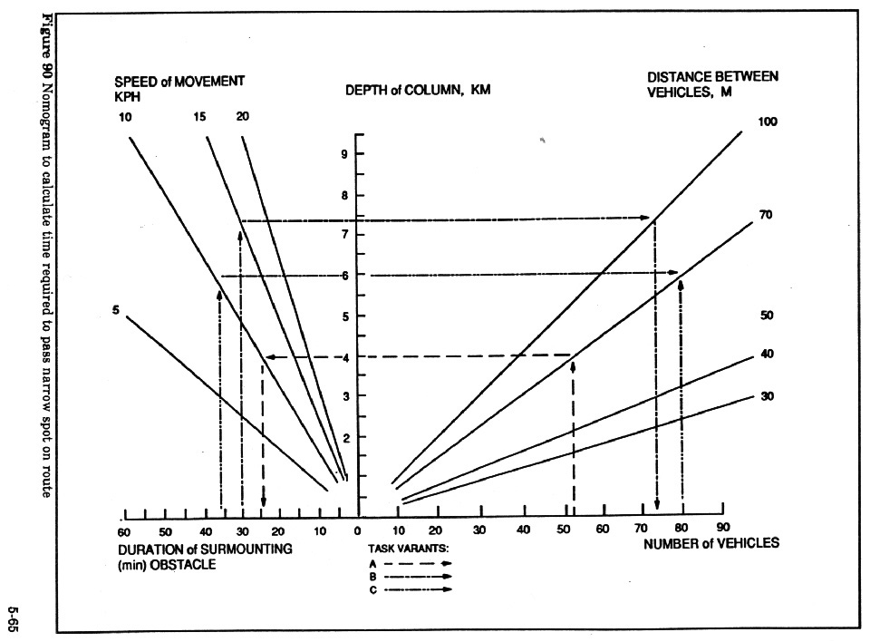
|
|
| |
Figure 91Nomogram to Calculate Time Required
to Pass a Difficult Section of Route
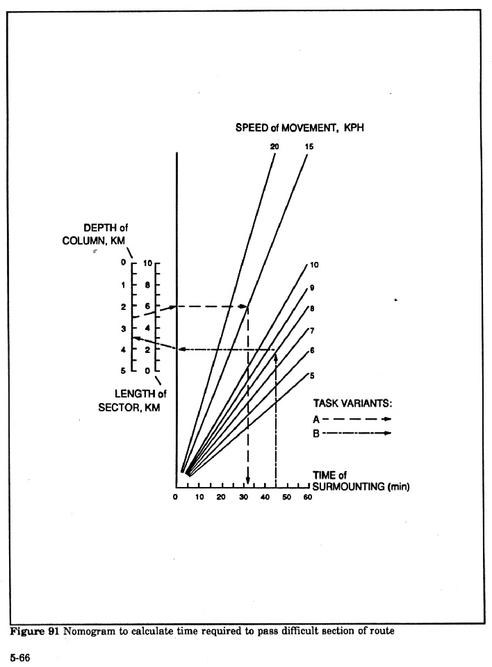
|
|
| |
(10) Calculation for Passage Times Across Start
Point )SL( by the Head and Tail of the Column
This calculation also determines the time for a column to pass a given point,
however, since there is no delay as with an obstacle, the time interval is
governed by the length of the column and its velocity. Since we are not
interested in the length of time the column requires, but the clock times the
head and tail cross, the equations yield time in military time.
The formula is:

where:
ti=SL crossing time of the head of the march column i in hours and minutes;
Ti-1=the time for passing the line by the tail of the leading march
column in hours and minutes; for the head of the first column this time is the
time specified for passing the line by the head of the entire formation, for
instance, by the column of the leading unit on a route;
di=the specified distance between the lead and the i march column in
km;
06=factor for converting hours into minutes;
V=average speed in km per hr;
t'i=the time for passing the line by the tail of the i route column
in hours and minutes;
Di=depth of the i column in km.
Example: to determine the passage time of the starting line or other
regulation point by the head and tail of the third column in a formation, when
the passage time of the cited point by the tail of the previous column is
21:15, the established distance between the columns in 1.5 km, the depth of the
column is 1.8 km and the movement speed is 25 km per hr.
solution:
t3=21:15 + ])1.5( x )60({ ÷ 25=21:15 + 0.04=21:19;
t'3=21:19=1.8 x 60 ÷ 25=21:19=0.04=21:23;
this means the third column in the march formation will pass the regulation
point with its lead at 21:19 and its tail at 21:23 hrs.
Example calculation using the nomogram Figure 92: The nomogram may be used to
speed up the calculation of the passage of a line by the head and tail of the
column. To determine the passage time of an initial line by the head and tail
of a march column 7 km line with the condition that the time for crossing the
line by the tail of the lead column is 20:20, the distance between the columns
is 5.5 km and the travel speed is 25 km per hr.
Solution: Draw a perpendicular line up from the horizontal axis, "Depth of
column or distance between columns" scale from the 5.5 mark to the
intersection with the "Average speed of columns -25" line. From this
point draw horizontal line to the "Time of passing point" scale and
read the result=13.3 or approximately 13 minutes. This is the time in which the
head of the stated column must pass the point after it is passed by the
previous column )at 20:00(. The time for passing a point by the tail of a
stated column is solved in a similar manner. For this draw a perpendicular line
from the 7 mark on the "Depth of column axis" to the intersection
with the "Average travel speed line - 25". From this point draw a
horizontal line to the "Time of passing point" scale and read the
result of 17 minutes. This means that this column must pass the control point
with its tail at 20:30.
|
|
| |
Figure 92 - Nomogram to Calculate Time Head
and Tail of Column will Pass Regulation Point

|
|
| |
(11) Calculation of Expected Time and Distance of
Probable Point of Contact with Advancing Enemy
Clearly this is one of the most important calculations Soviet commander's make
regularly during the course of combat. As the discussion of meeting engagements
in Chapters One and Two indicates, the commander's effort to control the flow
of battle focuses heavily on the relative times and place of introduction of
his second echelon versus the enemy's reserves, both of which are moving
forward.
The formula is:

where:
te=expected tome of meeting in hours;
D=initial distance between opposing groupings in km;
Vf=movement rate of friendly troops in km per hr;
Ve=movement rate of enemy forces in km per hr;
dl=distance from friendly initial position to expected point of
contact in km;
Example calculation: Determine the expected time of meeting and distance to
probable encounter line when enemy is located 63 km away, his average forward
speed is 25 km per hr, and average speed of friendly troops is 20 km per hr.
Solution: the equation yields distance of 28 km and time of 1 hr and 24 min.
Example using nomogram Figure 93: Determine the expected time of meeting and
distance to line of contact with enemy if at 18:00 the advancing enemy is
located at a distance of 64 km, his average speed is 15 km per hr, and friendly
troops are moving at 20 km per hr.
To use nomogram )variant a( find the marks "20" and "15" on
the "Speed of movement of own forces" and "Speed of movement of
enemy" lines respectively, draw a line through these points to
intersection with horizontal scale and read mark of 35. Then move downward
along the line shown by the dots to the intersection with the perpendicular
established from the "64" mark on the "Distance between our own
and enemy forces" scale. From this point of intersection draw a horizontal
line to the "Anticipated time of meeting" scale and read the
calculation result of 1 hr and 50 min. This will be the length of time from the
start time to meet the enemy. That means 18:00 plus 1:50 gives 19:50.
To determine the distance of the probable meeting line with the enemy (variant
b) from the result of 1 hr 50 min, draw a horizontal line to the intersection
with the speed line (ie at mark 20), which corresponds to the travel speed of
the friendly troops. From the obtained point, drop a perpendicular line to the
"Distance between friendly and enemy forces" scale and read the
calculation result of 36 km.
|
|
| |
Figure 93 - Nomogram to Calculate
Time and Disance to Point of Meeting Engagement
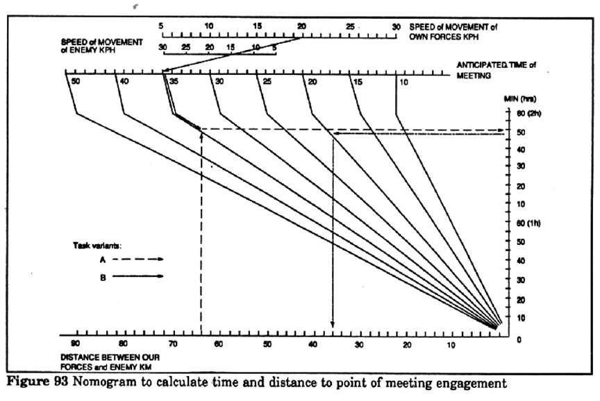
|
|
| |
(12) Calculation of Time Required for Advancing and
Deploying Sub-units to Change From Line of March into the Attack
Determination of the time a unit should begin to move for the advance from its
assembly area to the line of commitment into battle and assault on the enemy
position is a complex application of the basic time and distance formula. All
times are measured backwards from "CHE" hour, the moment the troops
hit the first line of the defending enemy's position. The total time from
beginning of movement in the assembly area is composed of the segments of time
while moving in each type of deployment, that is: line of attack, company
column, battalion column, and regimental column. It also includes the time it
takes to shift from one formation to the other and any time for halts and
delays en route. This is one of the most important and fundamental of tactical
calculations. The times for sub-unit movement are tied exactly into the times
for the artillery preparatory fire and air strikes.
The required given data are the distances between each of the deployment and
regulating lines, distance of the attack line from the enemy's forward line of
defense, distance of the start line from the unit assembly area, the average
speed of movement while mounted in the columns, the coefficient for speed
reduction during deployment actions, the speed of movement in attack formation,
the depth of the columns, and distance between first and second echelons of the
units. The set of formulas are:


|
|
| |
where:
ta=time for crossing final deployment into line of attack -
"Che" hour -in minutes;
Da=distance of line for going into attack formation from the forward
edge of the enemy position in km;
Va=rate of movement in attack formation in kph;
tr=time for crossing the line of deployment into company columns at
)"Che" - minutes(
Dr=distance of line of deployment into company columns from the line
of deployment into attack formation in km;
V=average rate of movement of subunits in mounted formation during march;
tb=time for crossing line of deployment into battalion columns at
)"Che" - minutes(;
Db=distance of line for deployment into battalion columns from line
of deployment into company columns in km;
trr=time for crossing the last regulation line or point prior to the
deployment into battalion columns;
Drr=distance of last regulation line from the line for deployment
into battalion columns;
ti=time for passing the start line at )"Che" - minutes(
Di=distance of start line from last regulating line in km;
tvit=time to begin movement of subunits in assembly area;
D=distance of start line from the last unit assembly area;
t'i=time for crossing the start line by the 2nd echelon
of units at )"Che" - minutes(;
Gk=depth of the mounted column of first echelon of units in km;
dk=distance between the tail of the first echelon and head of the
2nd echelon of the units in km;
The numbers 60 and 90 are coefficients for conversion of time in minutes for
the average speed of movement during the deployment of the units at each of the
lines. For example, the 90 shows that the average maneuver speed of the unit
during the actual deployment on a line decreases by a factor of 1.5 in
comparison with the speed of forward movement between the lines. Depending on
the concrete conditions and situation for movement on the terrain, this could
be some other factor.
To perform the calculation the required data may be entered into the table. The
result will be the planning data for start of forward movement and deployment
times for each shift of sub-unit columns. Since all times are measured backward
from "Che", the planner must remember to subtract the values
indicated in lines 12, 15, 18, 21, 23, and 27 from Che; and add the value for
time in line 30 to the time in 24 to obtain line 31.
|
|
| |
Figure 94 - Calculation of time to advance and
Deploy into the Attack from Line of March
CALCULATION OF TIME TO ADVANCE AND DEPLOY SUB-UNITS FOR
SHIFT INTO ATTACK FROM LINE OF MARCH
|
| No |
Initial data, values and calculations to
perform |
Units Precision |
Calculation variant |
| 1 |
2 |
3 |
| 1 |
2 |
3 |
4 |
5 |
6 |
| 1 |
Distance of attack line from enemy front line |
|
|
|
|
| 2 |
Distance of line to deploy into company columns from attack
line |
|
|
|
|
| 3 |
Distance of line to deploy into battalion columns from line of
company columns |
|
|
|
|
| 4 |
Distance of regulation line from line to deploy into battalion
columns |
|
|
|
|
| 5 |
Distance of regulation line from start line |
|
|
|
|
| 6 |
Distance of start line from the unit assembly )FUP(
area |
|
|
|
|
| 7 |
Movement speed into the attack |
|
|
|
|
| 8 |
Average speed during march |
|
|
|
|
| 9 |
Dept of first echelon march column |
|
|
|
|
| 10 |
Interval between first and second echelon columns |
|
|
|
|
| 11 |
)1( x 60 |
|
|
|
|
| 12 |
Time to cross line for shifting to attack )Che - min(
)11( ÷ )7(
|
|
|
|
|
| 13 |
)2( x 90 |
|
|
|
|
| 14 |
)13( ÷ )8( |
|
|
|
|
| 15 |
Time to cross line of deployment into company columns: )Ch - ( )12(
+ )14( |
|
|
|
|
| 16 |
)3( x 60 |
|
|
|
|
| 17 |
)16( ÷ )8( |
|
|
|
|
| 18 |
Time to cross line of deployment into battalion columns: )Ch - (
)15( + )17( |
|
|
|
|
| 19 |
)4( x 60 |
|
|
|
|
| 20 |
)19 ( ÷ )8( |
|
|
|
|
| 21 |
Time to cross regulation line )Ch - ( )18( + 20( |
|
|
|
|
| 22 |
)5( x 06 |
|
|
|
|
| 23 |
)22( ÷ )8( |
|
|
|
|
| 24 |
Time to cross start line )Ch - ( )21( + )23( |
|
|
|
|
| 25 |
)6( x 90 |
|
|
|
|
| 26 |
)25( ÷ )8( |
|
|
|
|
| 27 |
Time to start moving out of assembly area - 1st echelon )Ch - (
)24( + )26( |
|
|
|
|
| 28 |
)9( + )10( |
|
|
|
|
| 29 |
)28( x 90 |
|
|
|
|
| 30 |
)29( ÷ )8( |
|
|
|
|
| 31 |
Time for second echelon to pass start line )SL( )Ch - ( )24( -
)30( |
|
|
|
|
|
|
| |
(13) Calculation of the Time and Distance to the
Line of Contact
This method takes into consideration the many situational factors that are
ignored in the simpler formula and nomogram. In fact, there are so many
possible influences on the time the two sides will meet and hence the location
of meeting that a nomogram can only give a crude approximation of the answer.
With the use of computers or even hand calculators and an established procedure
such as that shown in this table it is possible to assess the influence of many
more factors.
The set of formulas is:
tv=}D + ])tn x Vn( + )tp x
Vp([{ ÷ )Vn + Vp(
Tn=t1 + t2 t3;
TP=t1' + t2' + t3'
where:
tv=expected time if contact with enemy in hours;
D=distance between forces of the two sides in km;
tn=total delay time for own force in hrs;
Vn=speed movement of own forces in km per hr;
tp=total delay time of enemy in hrs;
Vp=speed movement of enemy in km per hr;
lp=distance to expected line of meeting with enemy;
t1 )t'1(=delay - )time difference( start of
movement of one side versus other in hrs;
t2 )t'2=duration of halts of forces of each
side in hrs;
t3 )t'3(=duration of delay of forces due to
strikes by opponent en route in hrs;
Astronomical time of meeting enemy depends on complex conditions. Determine it
by adding the relative time obtained as a result of the calculation with the
astronomical time of the beginning of the approach of the opposing forces.
For example if the time to start march of own forces is 9PM the starting time
for the enemy is 10PM then astronomical time to start the approach is 9PM. If
the calculated time for meeting is about 2.5 hours then the time for meeting
would be 11:30.
Example problem: determine the expected time of meeting and the distance to
likely line of contact with the enemy and the duration of movement to that line
under following conditions:
- start time of own forces - 20:00 hrs;
- start time of enemy forces - 21:00 hrs;
- distance to enemy - 105 km;
The commander decides there will be a break of 20 minutes ).3( hr during the
advance. The plan is to delay enemy forces 30 -40 minutes ).6( hr. It is
assumed that during movement enemy will be required to take halts of 30 minutes
)0.5( hrs. The speed of movement of own forces is 28 km per hr. The speed of
movement of the enemy is 19 km per hr.
The answer is that contact will be at 11:20 at a distance of 84 km. Duration of
movement to meeting line is 3 hrs.
|
|
| |
Figure 95 - Form for Calculation of Expected time
and location of Meeting Engagement
CALCULATION OF EXPECTED TIME AND DISTANCE TO PROBABLY LINE OF
MEETING ENGAGEMENT
|
| No |
Initial data, values and
calculations |
Units Precision |
Calculation variant |
| Example |
2 |
3 |
| 1 |
2 |
3 |
4 |
5 |
6 |
| 1 |
Friendly force starts advance |
hr, min |
20:00 |
|
|
| 2 |
Enemy force starts advance |
hr, min |
21:00 |
|
|
| 3 |
Distance between opponents at start |
km )1.0( |
105 |
|
|
| 4 |
Delay in advance of friendly relative to enemy |
hr )0.1( if 1 < 2 |
-- |
|
|
| 5 |
Total duration of halts of friendly |
hr )0.1( |
0.3 |
|
|
| 6 |
Total duration of delays of friendly by enemy |
hr )0.1( |
-- |
|
|
| 7 |
Friendly force travel speed |
km/hr )1.0( |
28 |
|
|
| 8 |
Delay of enemy start relative to friendly |
hr )0.1( if 2 < 1 |
1 |
|
|
| 9 |
Total duration of halts of enemy |
hr )0.1( |
0.5 |
|
|
| 10 |
Total duration of delays of enemy due to friendly |
hr )0.1( |
0.6 |
|
|
| 11 |
Enemy force travel speed |
km/hr )1.0( |
19 |
|
|
| 12 |
)4( + )5( + )6( |
)0.1( |
0.3 |
|
|
| 13 |
)12( x )7( |
)0.1( |
8.4 |
|
|
| 14 |
)8( + )9( + )10( |
)1.0( |
2.1 |
|
|
| 15 |
)14( x )11( |
)1.0( |
40 |
|
|
| 16 |
)3( + )13( + )15( |
)1.0( |
153 |
|
|
| 17 |
)7( + )11( |
)0.1( |
47 |
|
|
| 18 |
Expected time of meeting )relative( )11( ÷ )17( |
hr )0.1( |
3.3 |
|
|
| 19 |
Duration of travel time to meeting line: )18( - )12( |
hr )0.1( |
3 |
|
|
| 20 |
Distance to meeting line: )19( x )7( |
km )1.0( |
84 |
|
|
|
|
| |
(14) Calculations of Expected Time and Rate of Overtaking
when Pursuing the Enemy
Naturally the commander hopes to use this calculation often! The initial data
are the distance between the enemy and friendly forces, the average travel
speed of friendly and enemy forces, or the ordered time to overtake him. The
formula is:
where:
to=time to overtake enemy in hours;
D=distance to the enemy in km;
Vn=friendly speed in pursuit in km per hr;
Vp=enemy speed in retreat in km per hr;
Example: Determine how much time it will take for forces to overtake a
retreating enemy when the distance to him is 20 km, his rate of retreat is 10
km per hr, and the rate of advance of friendly forces is 25 km per hr.
Solution: to=20 ÷ )25 - 10(=1.3 hrs ;
Determine the pursuit speed required to enable friendly forces to overtake
enemy in 45 min, when he is 15 km away and his travel speed is 12 km per hr.
Solution: Vn=))15 + 0.75( ( 12) ( ÷0.75=33 km per hr.
Examples of calculations using the nomogram Figure 96:
Determine the expected time to overtake enemy when his distance is 30 km, his
travel speed is 20 km per hr, and the speed of pursuit is 28 km per hr. In the
calculation )variant a( establish a perpendicular line from the "30"
mark on the "Distance between friendly and enemy forces" scale. Then
draw a line through the "28" mark on the "Friendly forces travel
speed" and the "20" mark on the "Enemy travel speed"
scale to its intersection with the horizontal upper axis. From this point draw
a line down as shown by the dots to the intersection with the previously set
perpendicular line. From the point of intersection draw a horizontal line to
the right and read off the result of 3 hrs and 45 min on the "Expected
encounter time" scale.
Determine the required pursuit speed to intercept the enemy in 1 hr and 20 min,
when the enemy is at a distance of 40 km and is traveling at a speed of 5 km
per hr.
In calculation )variant b( establish a perpendicular line from the
"40" mark on the "Distance between friendly and enemy
forces" scale to the intersection with the horizontal line, drawn from the
1 hr and 20 min mark on the "Expected encounter time" scale. From the
meeting point draw a line, as shown by the dots and dashes, to the horizontal
scale. Draw a line through the point of intersection of this scale and the 5
mark on the "Enemy travel speed" scale and continue it to the
intersection with the "Friendly force travel speed" scale, where the
result is 35 km per hr. This means that the pursuit speed must he at least 35
km per hr.
|
|
| |
Figure 96 Calculation of Expected
Time and Rate of Overtaking when Pursuing the Enemy:

|
|
| |
(15) Calculation of the Work Time Available to the
Commander and Staff for Organizing Repulse of Advancing Enemy Forces:
This is obviously a critical issue in meeting engagements and encounter battle.
It is also relevant to defensive situations when preparing fire on the
attacker. The method is designed to determine the time the commander and staff
will have to organize the enemy's defeat by firing on the advancing forces
relative to the distance to the enemy, the speed of his advance, the effective
range of friendly weapons and the time required to prepare the sub-units to
fire. In this example it is assumed that the enemy will be taken under fire
beginning at the maximum range of the firing weapons. The formula is:
where:
t=time available for commander and his staff to organize repelling the
advancing force in minutes;
D=distance to advancing enemy km;
d=max range of friendly weapons km;
60=conversion factor hours to minutes;
Ve=rate of enemy advance kph;
tp=time required to prepare subunits to destroy enemy with fire in
minutes;
Example: Determine how much time is available for the commander and staff to
organize destruction of the advancing enemy if it is located at a distance of
25 km, his average speed is 15 km per hr, the effective range of the weapons is
12 km., and the time for preparing the sub-units is 03 min.
Solution: t=} (25 - 12) x 60 ÷ 15{ - 30=22 min.
Example calculation using the nomogram Figure 97: Determine the time the
commander and staff spend in organizing the destruction of an advancing enemy
if he is 15 km away, his rate of advance is 12 kph, the effective range of
friendly weapons is 6 km, and the sub-unit preparation time is 20 min.
Solution: Mark the points "15" and "6" on the "Enemy
distance" and "Effective range of friendly fire" scales,
respectively. Draw a straight line through them to intersection with the
vertical axis. From this point draw a horizontal line to the "Enemy
advance speed - 12" line. From that point drop a perpendicular line to the
horizontal axis and make a mark on it. Then draw a line through that mark to
the "20" point on the "Time for preparing the sub-units for
combat" scale. At the point of intersection of this line with the
"Commander and staff work time" scale read the result of 25 min.
|
|
| |
Figure 97 - Nomogram to Calculate
Time Available to plan fire on advancing Enemy

|
|
| |
(16) Calculation of Length of Time to Operate
Command Post in a Single Location
One of the important calculations performed by the operations staff is to
determine the duration of time a command post can remain at one location during
an offensive and still keep up with the advancing troops. Obviously, the longer
the CP can remain in place the more work that can be done and less time lost to
transfers, however, the CP must not lag too far behind the forward edge of
troops, if the commander is to exert direct supervision and control. The
required data are the established maximum and minimum distance norms of the
command post from the forward edge of battle, the rate of movement for the
leading troops, the movement rate for the command post, and the time required
for loading up and deploying the command post for each move. The calculation
would be similar for any other entity that should remain between maximum and
minimum distance from another, for instance rear service installations. The
formula is:

when D < d
t=length of time available for work at the CP in one location;
D=maximum distance of CP from forward edge in km;
d=minimum distance of CP;
Vs=rate of movement of leading sub-units;
Vc=rate of movement of CP during its relocation;
60=coefficient for conversion of hr to min;
tbd=duration of loading and unloading time for CP.
Example problem: Determine the working time for a CP when maximum distance
is 7 km, minimum distance is 1.5 km, rate of movement for units is 4 kph, rate
of movement for CP is 25 kph, and time to load and deploy is 15 min.
Answer is 54 min
|
|
| |
Figure 98 - Calculation of Duration of Operation of
CP in one Location
CALCULATION OF DURATION OF OPERATION OF CP IN ONE LOCATION
|
| No |
Initial data and values to be
determined |
Units |
Calculation variant |
Remarks |
| Example |
2 |
3 |
| 1 |
Permissible distance of CP from front |
km |
7 |
|
|
|
| 2 |
Minimum distance of CP from front |
km |
1.5 |
|
|
|
| 3 |
Sub-unit rate of advance |
km/hr |
4 |
|
|
|
| 4 |
Command post travel rate |
km/hr |
25 |
|
|
|
| 5 |
Time to deploy and break down CP |
min |
15 |
|
|
|
| 6 |
Duration of operation in one location |
min |
54 |
|
|
|
|
|
| / |
(17) Determination of Quantity of Various Weapons,
Reconnaissance, Support, Communications etc. for Task Performance
This general technique is applicable to a wide variety of activities in which
it is desired to know what the overall effectiveness of a group of agents will
be when the probability of success of an individual agent is known. First one
calculates the action of the number of identical equipments, and then
determines the total effectiveness or total requirement for the systems. the
initial data for the calculations are information about the number of available
systems, the assigned degree of success for each, the effectiveness of the
systems )which is expressed in probability of mission fulfillment or by the
mean value of the applied damage to a particular target.( A single system also
means a complex of systems combined into a whole unit. Such data, for instance,
are the probability of target destruction, the man damage applied to an enemy
target, the reliability of a communications channel, the probability of enemy
target detection, the probability of the flawless operation of a water crossing
for a specific time interval, the probability of overcoming the anti-air forces
of the enemy and so on. These data may be obtained on the basis of the results
of studies, from statistical data nd from tactical and technical
characteristics.
The formulas for calculating the degree of mission fulfillment by a designated
number of systems is expressed through mission fulfillment probability:
and through the mathematical expectation )mean value( of damage:

where:
Pn=probability of mission accomplished by a homogenous group of
weapons;
P1=same by a single system;
Mn=average )mean( value of damage inflicted on the enemy by a group
of systems;
M1=average value of damage inflicted on the enemy by one system;
n=quantity of available systems.
The formulas for computing the required number of systems when the
effectiveness of the systems is expressed by probability of task performance
is:
when Pn < P1

when it is expressed by the mathematical expectation )the mean value( of
the inflicted damage, the formula is: when Mn < M1

The formula for calculating the effectiveness of different systems
fulfilling a common mission is :

where Pnis the overall effectiveness of systems used or in other
words the likelihood of fulfilling the mission, and the individual
"P"'s are the effectiveness measures of each system being summed for
the task.
Example: Determine probability of spotting an enemy target with combined
use of 3 reconnaissance systems, if their effectiveness expressed as the
probability of detection of enemy target is:
P1=0.4; P2=0.6; and P3=0.8
Solution: Pn=1 - )1 - 0.4( x )1 - 0.6( x )1 - 0.8(=0.95 or
approximately 1.
Example calculations using nomogram Figure 69: Determine the probability of
enemy target destruction with a strike against it by three systems when the
probability of target destruction by a single system of the particular type is
0.4.
Solution: )variant a( Draw a perpendicular from the "3" mark on the
"Required number of systems" scale to the intersection with the
"Probability of mission fulfillment by one system - 4" curve. From
this point draw a horizontal line and on the "Probability of mission
fulfillment by a group of systems" scale read that the probability of
target destruction by three systems is 0.78.
It is possible to determine the reliability of communications in a link which
consists of two channels )n=2(, when the reliability of each channel is 0.6.
From the nomogram, the probability of faultless operation of communications in
this instance will be 0.84.
It is possible to evaluate the effectiveness of using four similar
reconnaissance systems to detect an enemy target in an assigned region when the
probability of detection by one system is 0.5. According to the nomogram, the
probability of target detection by four systems will be close to one (.94.
Determine how many weapons systems must be assigned to inflict no less than 90%
damage an enemy target, when the average damage inflicted byu a single system
is 70%.
Solution: Draw a horizontal line from the "0.9" mark on the
"Probability of mission fulfillment by a group of systems" scale to
the intersection with the "Probability of mission fulfillment by a single
system - 0.7" curve. From the intersection point drop a perpendicular line
and on the "Required number of systems" scale find the result - 2.
This means two systems must be used to achieve the assigned damage.
It is possible to determine the required number of communication channels to
provide for 90% reliability when the reliability of a single channel is 0.6.
From the nomogram it appears that at least three channels are required to
ensure this reliability.
From these examples it is evident that the technique may be used for
calculating a wide range of direct and inverse problems associated with the use
of various forces and means. With proper additional factors this method may
also be used to calculate rapidly the effectiveness and required number of
forces and systems when taking into account also probable enemy
countermeasures.
The formulas for calculating the effectiveness of forces and means with
consideration for probable enemy countermeasures are:

where:
Pn=the probability of mission fulfillment by a group of systems;
P1=the probability of mission fulfillment by a single system of this
type;
Q=the probability indicator of the enemy countermeasure ;
n=the number of forces and means of the given type;
Mn=the mathematical expectation of the damage inflicted by a single
system of this type'
Example calculation: To determine the probability of mission fulfillment by
five weapons systems when the probability of target destruction by a single
system is 60%, while the probability of successful enemy countermeasures is
50%.
Solution: Pn=1 - )1 - 0.6 x 0.5(5=1 - )1 -
0.3(5=0.83.
|
|
| |
Figure 99 - Nomogram for Calculating
the Combined Effectiveness of several Systems
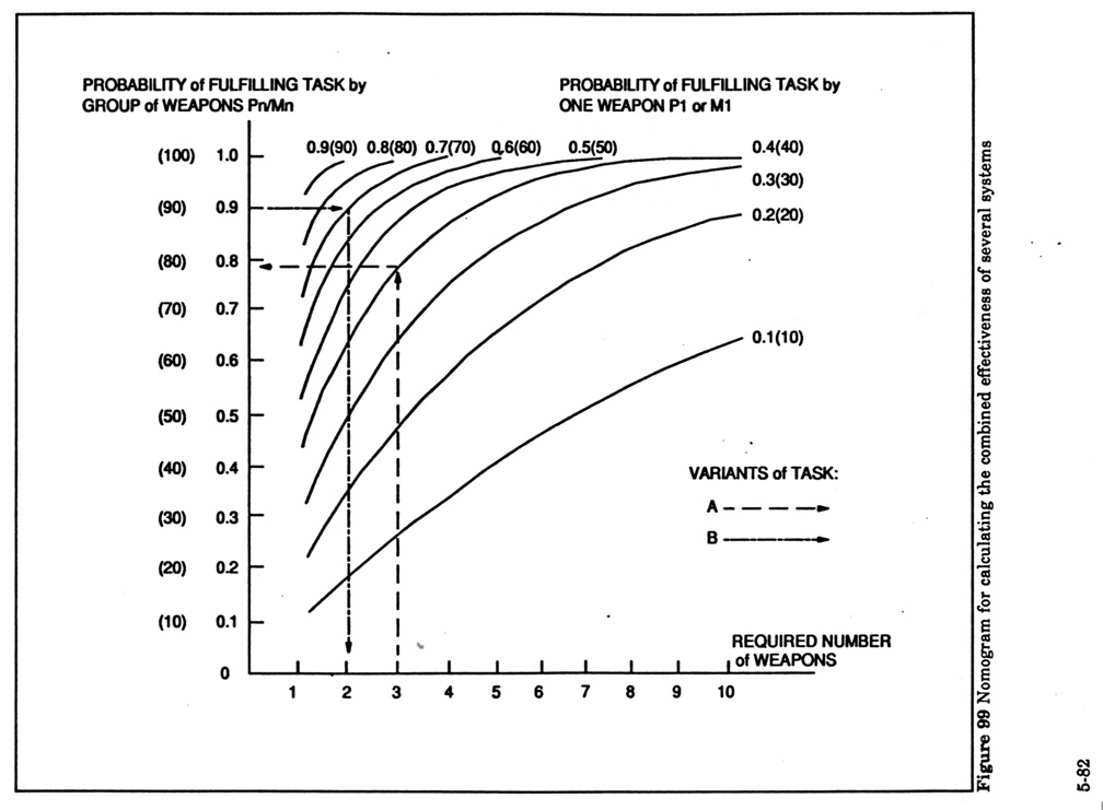
|
|
| |
(18) Modeling battle(4)
There is much discussion in the Soviet literature about the theory of
development of coefficients of comensurability. The coefficient is designed to
make it possible to aggregate the effective contribution of various weapons to
a combined arms battle into a composite score for each side. This makes the
measurement of the correlation of forces relatively simple, ie. only one number
for each side rather than the long list of individual types of weapons found in
the standard tables of correlation of forces. However, what sounds simple in
theory is quite difficult in practice. Soviet authors point out that even
within types of weapons such as tanks or artillery the "proving ground
scores" assigned on the basis of technical/tactical characteristics may
not be true reflections of the actual value of the weapon to the commander in
all the diverse conditions of real combat. When it comes to establishing a
uniform score that will place tanks, artillery, aircraft, and small arms, etc
on one scale; a lot of judgment is involved. There is some argument for two
different methods, one would develop a "average" score for each
weapon reflecting its varied value in different circumstances, and the other
method would establish a single theoretical value number and then provide
situation modifiers to be applied to account for each actual set of combat
conditions. We do not have available an actual set of Soviet "utils"
as they call their weapons scores. The following table is taken from a Soviet
article, but the scores are purely hypothetical for educational purposes.
Nevertheless, the following method represents a typical Soviet approach which
may be used by American officers with an appropriate set of "utils".
|
|
| |
Figure 100 - Coefficients of
Comensurability
COEFFICIENTS OF
COMENSURABILITY
|
| Nationality |
Type of combat equipment |
Coefficient of comensurability |
| Country A |
Tank 5 |
1.0 |
| Tank 6 |
1.12 |
| Tank 7 |
1.5 |
| APC |
1.6 |
| AT gun |
0.3 |
| Country B |
Tank 06 |
1.02 |
| APC |
1.4 |
| PTRK |
0.95 |
| AT gun |
0.3 |
| Country V |
Tank 1 |
1.09 |
| APC |
0.45 |
| PTRK |
0.78 |
| RPG |
0.12 |
|
|
| |
Figure 101 - Expected
Losses
EXPECTED LOSS IN
COMBAT EFFECTIVENESS
|
| Nationality of forces |
Defense |
Offense |
Meeting battle |
| Prepared |
Non-prepared |
On prepared line |
On unprepared line |
| Country B |
55 |
45 |
30 |
35 |
40 |
| Country V |
60 |
50 |
35 |
40 |
45 |
|
|
| |
The mathematical expectation of the level of destruction
of a side from fire and strikes of artillery and aviation )M( in the experience
of the Great Fatherland War could reach on defense to 04-06% and on the offense
to 02-03%. The losses of combat effectiveness due to destruction in various
types of combat is shown in the table of expected losses. Another Soviet source
gives 03% loss as the critical break point for attackers and 04% loss as the
typical break point for defenders. Of course the effect of losses on unit
combat effectiveness depends heavily on the rate of loss and the size of the
unit. One more indicator is the coefficient of superiority )Kp( of
the defenders over the attackers, which in the experience of combat typically
is three times.
The possibility of sub-units for destruction of the enemy during the course of
accomplishing their combat missions is calculated according to the following
formulas:
|
|
| |
a( in offense:

b( in defense:

where:
Ks1, Ks2, Ksp=coefficients of comensurability
of combat means of units of country A;
Kb1, Kb2, Kbp=coefficients of comensurability
of combat means of units of country B or V;
i=quantity of combat means of given type;
Z1, Z2=level of destruction at which the unit loses
combat effectiveness;
M=mathematical expectation of the level of destruction due to artillery and
aviation fire;
Kp=coefficient of superiority of defender over attacker;
S=combat capability of the sub-unit.
For calculations of combat capability during meeting engagement )battle( use
formula )1( but for the coefficient of superiority of defender over attacker
use 1.
Example calculation: The tactical situation; a tank platoon of country A )with
tanks 7( with motor rifle section in a APC has the mission of attacking from
the march to destroy defending section of country B.
Initial data for the calculation:
- a. type of combat action is attack;
- b. model of combat means of the sides, their quantity and coefficient of
comensurability calculated qualitative indices, are shown in table of
comensurability.
The attackers:
- tanks "7" Ks1=1.5, and quantity, i=3;
- APC, Ks2=0.8, and quantity, i=1.
Defenders:
- APC, Kb1=1.4, and quantity i=1;
- AT gun, Kb2=0.3, and quantity i=3;
c. the mathematical expectation of the level of destruction of the defenders in
the time of artillery preparatory fire and attack support fire is M=0.4;
d. losses of the sub-unit during the time of approach to the line of going over
to the attack must not exceed Z1=0.3;
e. level of destruction of the defenders at which they loose combat
effectiveness is found in the table of expected loss of effectiveness, Table 2,
Z2=0.55;
Taking the initial data and using formula 1 to create a mathematical model of
the battle gives the following:
- Sn=}])1.5 x 3( + )0.8 x 1([ x ]1 - )0.3 + 0.55 - 0.4([{ ÷ }3
])1.4 x 1( + )0.3 x 3([ x )1 - 0.4(=0.7
Analysis: If Sn is greater than or equal to 1, then the sub-unit
will fulfill its mission, if )as in this example( the Sn is less
than 1, then the defender with his forces will be superior. This means that it
is necessary to raise the capability if the force to achieve likelihood of
accomplishing the mission.
Decision: Reenforce by fire the platoon on the march from a range of 0002
meters to destroy the enemy APC, and after that conduct fire on the AT gun.
The problem may be decided by means of mathematical modeling of battle:
- Sn1=}])1.5 x 3( + )0.8 x 1([ x )0.3 + 0.55 - 0.4({ ÷ )3 x 1.4
x )1 - 0.4((=1.19;
In other words, the APC will be destroyed.
- Sn2=})1.5 x 3 + 0.8 x 1( x )1 - )0.3 + 0.55 - 0.4({ ÷ }3 x
0.3 x 3 x )1 - 0.4({=1.9.
Outcome: Attacking from the march with forces of three tanks and APC to destroy
an APC and then a AT gun. The line of going over to the attack is designated in
accordance with the characteristics of the terrain, but not closer than 0002
meters from the forward edge of the enemy defenses.
As is evident from the example, the conduct of the calculation is difficult
work demanding a significant amount of time and corresponding conditions. If
the commander has an electronic calculator he could work out the answer
quickly.
What is not evident is to what level of aggregation this method and these
formulas may be taken without loosing validity. The given example illustrates
duels and very small unit combat. With the use of computers it would be
possible to calculate combat at the level of a full regiment or even division
but so many other factors enter in and effect combat outcomes at that level
that a simple formula is no longer valid.
|
|
| |
(19) Calculation of Strike Capability of
Sub-units(5)
This method is designed to calculate the expected depth of penetration of a
unit on the offensive as a measure of its strike capability, or, in reverse, to
forecast the ability of a unit of given combat capability to achieve the depth
of penetration required in its mission. The initial data for the calculation
includes the composition of the attacking and defending units, the conditions
of combat and combat potentials with calculated losses of the sides and also
the designated critical level of losses necessary to cause unit failure.
The critical figure is considered to be the loss at which the sub-unit losses
its combat capability and cannot continue the kind of action it was performing
without re-enforcement. The calculation is made over the width of the front of
the attacker and the designated area of the defense. See the section on
modeling battle for more discussion of the theory and use of the critical level
of loss as an indicator in forecasting and modeling combat. Together these
formulas may be used to determine the initial data on the three measures of
effectiveness described in Chapter One as those deemed critical for assessing
and forecasting battle outcomes.
The formula for calculating tbe expected depth of penetration follows:
when:
YN )1 - PN ( < )1 - PNK( and
Yo )1 - Po( < PoK(
where:
NN, No=number of units of attackers and defenders,
measured in combat potentials )"utils"(;
PN, Po=expected losses of the units of each side up to
the arrival at the immediate mission line;
PNK, PoK=critical loss of a unit of
attacker and defender;
FN=width of front of attack in km;
Fo, Go=width of front and depth of the defender's area in
km.
YN, Yo=composition of the units of each side as a
percentage of unity 001%.
K=coefficient of combat effectiveness of the defending side. )This is the same
as Kp in the formulas for modeling battle.
Sample calculation: Determine the expected depth of penetration of attacking
unit whose combat potential at 100% measures 150, during an attack on a enemy
having a combat potential of 194 and a manning of 85%, if the attackers losses
in the immediate battle reach 10% and the defender's losses reach 40%. The
critical loss for the attacker is 50% and for the defender is 70%. The attack
is conducted on a front of 5 km. The defending unit occupies an area of 8 km
wide and 10 km deep, and the coefficient of effectiveness of the defender is
2.5.
Solution:

This should be 150 (1.0 (1-0.1) - (1 - 0.5)) x 8 x 10
over 194 (0,85 (1 -.04) - (1 - 0.7) ) x 5 x 25=9.5
This means the attacking unit can be expected to succeed in reaching a depth of
9.5 km in the defender's position. The Soviet author does not indicate the
scale of this combat, and in fact uses the term for sub-unit )ie. a battalion
or smaller(, but from the dimensions of the combat area )8 km by 01 km( we may
assume this is a regiment attacking of a brigade frontage to the full depth.
If we use the same formula to evaluate battle at division level we may assume
"utils" of NH=800 for attacker and NO=700 for
defender and the following other values for variables:
YN=90%; YO=80%; PN=0.1%; PO=0.4%;
K=1.5;
PNK=0.5%; POK=0.7%;
FO=20 km; GO=30 km; FN=15km;
The resulting equation is as follows:

Again, the numbers should be 800, 20, 30,700, and 15 -
the computer reverses many numbers
With these assumptions the attackers may be expected to achieve a depth of
penetration of 53 km.
Using the same formula to evaluate battalion scale combat we may assume both
sides have "utils" of 40, the defender has a superiority coefficient
of 2.5 and the widths are 4, 2, and 1.5 km. Then the formula yields the result
as a penetration of 3.2 km. These are not unreasonable depths for the types of
units being considered.
|
|
| |
(20 ) Calculation of the Width of Main Attack
Sector
There are several different ways to determine the possible, desired, or
required width of the main attack sector depending on the purposes and
criteria. The following is one quick way to calculate the relationship between
the width of a strike sector and the total width of zone in relation to the
correlation of forces in the strike sector and the total correlation. For these
calculations the correlation of forces may be calculated in terms of
"utils" or in terms of some other aggregate measure based on the
quantities of forces and means of the two sides. The following formula applies:

where:
Wm=width of strike sector;
Wo=total width of zone;
Co=overall correlation of forces;
Cm=correlation of forces in strike sector;
Cs=minimum desired correlation of forces in rest of zone excluding
strike sector.
Example calculation: Given the width of full zone of action is 120 km, the
overall correlation of forces is 1:1, the correlation of forces in the strike
sector is to be 3:1, and the minimum allowable correlation of forces in the
rest of the area is 0.5:1; determine the possible width of the strike sector.
Solution: Wm=120 )1 - 0.5( ÷ )3 - 0.5(=24 km.
Example calculation: Determine the correlation of forces possible in the strike
sector given that the total width of zone is 400 km, the overall correlation of
forces is 0.8:1, width of strike sector is desired to be 120 km, and the
minimum correlation of forces allowable in the rest of the area is 0.5:1.
Solution: The formula may be restated as Cm=Wo ÷
Wm )Co - Cs( + Cs ; inserting the
given data produces a result of 1.5 as the possible correlation of forces for
the strike sector. The commander may then decide on several alternatives such
as narrow the strike sector, weaken the non-strike sector even more, bring in
reinforcements, or weaken the defenders with preliminary artillery and air
bombardments. Having done the initial calculation the commander may use the
same formula in various ways while deciding on alternatives. For instance, to
determine the required reenforcement to obtain a desired higher correlation the
relationship is C=) 1.25 - 0.8( ÷ 0.8 x 100=56.25%, that is by reinforcing
by 56% the correlation in the overall area may be raised from 0.8 to 1.25 to 1.
|
|
| |
(21) Calculation of Required Destruction of
Enemy
Another calculation related to the preceding is to determine what damage should
be inflicted on the defender prior to the attack in order to bring the
correlation of forces into the desired range, considering that there will be a
given amount of loss on the friendly side as well. The formula is as follows:
100 not 001
where:
M=required level of destruction of enemy in percent;
CN=beginning correlation of forces;
CT=required correlation of forces;
P=forecast friendly losses from enemy action in percent.
Example calculation: In the break through sector regrouping of forces may bring
the correlation of forces to 2:1, however for successful break through we need
to bring the correlation up to 4:1 by means of initial artillery and air
bombardment inflicting losses on the defenders. Determine what level of damage
must be inflicted, if it is expected that the enemy will also inflict 30% loss
on the attacking strike grouping.
Solution: M=100 - 2 ÷ 4 ) 100 - 30 (=65%. Assume that the initial
"utils" of the attackers are 2000 and the defenders are 1000 for a
correlation of 2:1. The enemy will inflict 30% losses bringing the attacking
force to 1400 while the attackers must inflict 65% losses to bring the defender
to 350 "utils" to achieve the 1400/350=4:1 ratio. For more rapid
calculation of this relationship to determine the required losses to inflict
one may use the following nomogram )Figure (. The nomogram is based on the
above formula. The example shown is for the same situation. Enter with the
correlation of forces 2 on the bottom left and draw vertical line to the
correlation of forces 4 line, then a horizontal line across to the 30% loss
line and again vertical down to read the required enemy loss of 65%.
|
|
| |
Figure102 - Nomogram to Determine Required
Losses to Achieve Correlation of Forces

|
|
| |
(22) Calculation of Rate of Advance in Relation to
Correlation of Forces(6)
Various Soviet articles have discussed the concept of the relation of advance
rates to the correlation of forces of the sides. The relationship is complex
and also depends on several other variables. Evaluation and analysis of the
actual correlations of forces achieved in various operations of World War II
and recent local wars shows that a single norm for the correlation of forces
and means does not exist, but it all depends on the concrete conditions.
Nevertheless sufficient figures to make approximate calculations can be
developed, especially for academic and training purposes. The actual rate of
advance, V, in km per day may be related to a coefficient reflecting the
influence of the correlation of forces, KC, in an equation such as
V=140 x KC. In this the number 140 represents the collected
resulting effect of variables acting in the area, for instance the Western TVD
to give a practical maximum technically possible speed of movement for
mechanized forces in km per day and also an indicator characterized by the
influence of terrain, engineer obstacles, time of year, length of daylight,
etc. The factor KC is a coefficient depending on the correlation of
forces of the sides. This approximate relationship can be shown in a graph.
Analogous graphs can be made for other theaters and conditions. The formula
together with the graph is used to evaluate the formation and determine the
correlation of forces required to achieve a required rate of advance or in
reverse the expected rate of advance for a given correlation of forces.
Example calculation: A given strike group has a planned average rate of advance
of 40 km per day. Determine what the required correlation of forces superiority
is to achieve this rate.
Solution: Taking the formula V ÷ 140=KC or 40 ÷ 140=0.29.
Enter 0.29 on the scale for KC in the nomogram and draw a horizontal
line to the curve and then a vertical line down to the scale of correlation of
forces scale. This shows a required correlation of about 3.4:1 for the strike
sector.
Example calculation: In the zone of action of the strike group we have created
a 2.5:1 superiority in correlation of forces. Determine the approximate tempo
of advance.
Solution: From the nomogram read that the correlation of 2.5:1 corresponds to a
K factor of 0.13. Then using the formula V=140 x 0.13=18.2 km per day advance
rate.
Another approach is to use the following formula to calculate a factor
corresponding to the K factor in the previous method. In the following nomogram
the rate of advance is related also to movement distance, terrain type, length
of the operation and a theoretical maximum movement speed. These variables are
joined into a single factor according to the equation: F=D ÷
KTVmax where:
D=distance )depth( of operation;
K=terrain coefficient )1.25 - level; 1.00 - rough-level; .75 - rugged hills;
.75 - urban; .50 - mtns.(
T=time required for operation in days and fractions of days;
Vmax=theoretical speed in km per day.
According to this nomogram, to achieve a depth of advance of 03 km on level
terrain in one day with a theoretical maximum speed of 06 km per day requires a
superiority in correlation of forces of 4:1. With a correlation of forces of
3:1 on rough-level terrain and a theoretical maximum speed of 50 km per day in
two days the force may advance 20 km.
|
|
| |
Figure 103 Nomogram relating correlation of
forces to rate of advance (1)

|
|
| |
Figure 104 Nomogram relating correlation of
forces and rate of advance (2)
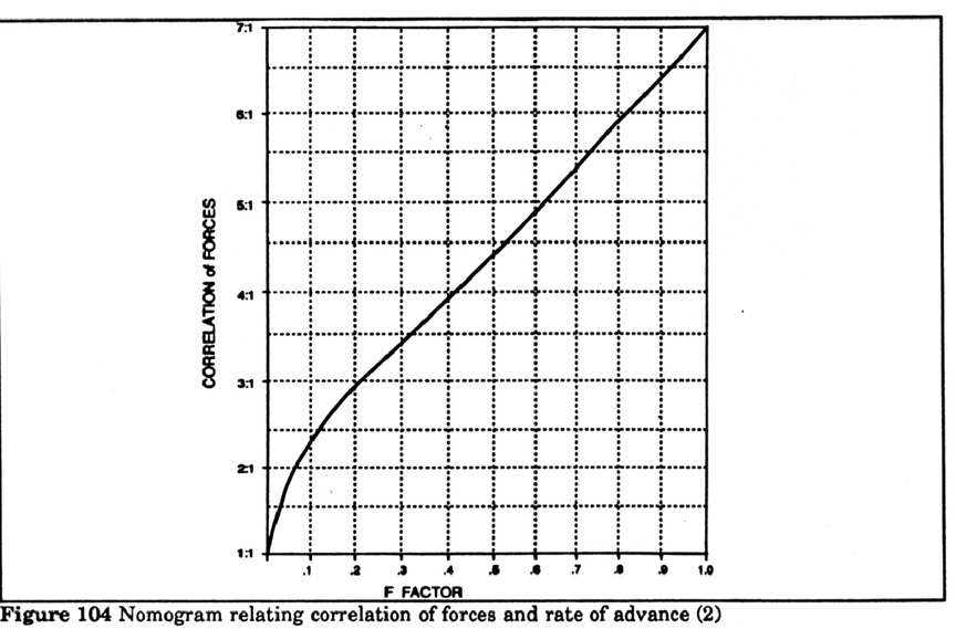
|
|
| |
(23) Determine the Possible Friendly and Enemy
Losses in Relation to the Correlation of Forces and Rate of Advance
A simplified expression of the relationship between attrition and the
correlation of forces may be shown with a nomogram. In actuality many factors
influence this relation, however, for general planning at front level
the averages shown in the nomogram may be sufficient. This nomogram is built
with the following assumptions.
1. The attacker needs a 3:1 advantage represented by the line at 45 degrees to
break even and have the same loss rate as the defender.
2. The losses to each side are related to the force ratio in a relatively
simple and direct way, but the greater the force ratio advantage and the longer
the time interval the larger the difference in attrition will be. So losses
accumulate faster for the side with the disadvantage in forces;
3. For an army size force the losses are about .5% per day when the correlation
of forces in 1:1
|
|
| |
Figure 105 Force attrition
nomogram - army

|
|
| |
Figure 106 Force attrition nomogram
front

|
|
| |
(24) Determine the Required Amount of Manpower and
Weapons for Bringing Sub-Units back up to Sufficient Strength to Restore their
Combat Capability
This calculation is made to determine how many men and weapons are needed to
restore the sub-unit or unit to combat capability sufficient to accomplish the
mission. It is not expected that the replacements will restore the sub-unit to
its original full strength, but just to the necessary ratio of correlation of
forces and means between the two sides. The mission was determined in the first
place on the basis of a calculated correlation of forces and means deemed
sufficient )such as 3:1(. Since both sides have suffered losses the quantity
required to restore the original favorable correlation will not equal the loss.
The basic data needed for the calculation are information on the original full
strength of the troops of the two sides, the losses sustained and the
superiority ratio of correlation of forces and means required for carrying out
the task. The results of the calculation represent the quantities necessary to
restore the force to its combat capability. Combat capability in this case
means sufficient strength to accomplish the mission. Obviously this is one of
the most important calculations Soviet commanders must make during combat. The
formulas for the calculation are:
Mi=Ci - Ai ÷ Bi ;
Ai=)nf Pf( x Nf ;
Bi=)ne -Ne Pe( x Ne ;
mi=Bi x Mi
where.
M=index of the reduction of combat capability in terms of the required ratio of
manpower and weapons for the execution of the mission;
Ci=required degree of superiority ratio for a particular type of the
i type of weapon;
Ai=availability remaining on hand quantity of weapons of a
particular type i of own forces;
Bi=availability of remaining number of weapons of a particular type
i for enemy forces;
nf )ne(=initial full strength of own troops )enemy
troops( by type i of weapons pers/ proportions;
Pf )Pe (=losses of own troops )enemy troops(
pers/proportions;
Nf )Ne (=TOE number of weapons of a particular type i of
own forces )enemy forces(;
mi=number of weapons of a particular type which are required for the
restoration of own troops combat capability.
If M is less than 0 then the calculation is no longer performed since the
filling out of the forces and means is not required to restore combat
capability. This method may be used both in calculating the number of various
types of combat equipment, as well as in calculating the correlated
quantity/quality indicators.
What these formulas mean essentially is that M is an index showing the reduced
combat capability of friendly forces in terms of the change in the correlation
of forces resulting from the differential losses by the two sides. It is equal
to C )the required correlation of forces ( minus the actual ratio )correlation(
of forces.
The term "A" is the remaining quantity of forces or means of the
particular type for friendly forces and it is equal to the initial strength
minus the product of the friendly initial strength times the losses to friendly
forces all times the TOE strength.
The term "B" is the same thing for the enemy forces.
Then m is the quantity of the forces or means required to restore the initial
favorable )required( correlation and it is equal to the remaining strength of
the enemy )B( times the M index of reduced combat capability )deficit in
correlation(
Example calculation using the table: Determine the required number of tanks and
guns to re-equip a sub-unit if the required level of superiority is 2.5:1, the
initial full strength of own troops was 88% )0.85(, the losses of own forces in
tanks is 40% )0.4(, the initial full strength of the enemy was 60% )0.6(, his
losses in tanks are 40% )0.4(.
Solution: Entering the data in the table we find that to resupply the sub-unit
and restore its combat capability requires 2 tanks. Replacements of guns are
not required since, given the losses on both sides, the required level of
superiority necessary to fulfill the mission is preserved.
|
|
| |
Figure 107 Form for the Calculation of the Required
Amount of Personnel
| CALCULATION OF FORCES AND MEANS TO RESTORE
COMBAT EFFECTIVENESS |
| No |
Initial data, values and operations to be
determined |
Unit (Accuracy) |
Forces and equipment |
| Tanks |
Guns |
Mortars |
BTR |
Etc |
| 1 |
Initial full strength of friendly forces |
percent |
0.85 |
0.7 |
|
|
|
| 2 |
Friendly forces losses |
percent |
0.4 |
0.2 |
|
|
|
| 3 |
Tabular volume of friendly force equipment |
units |
25 |
32 |
|
|
|
| 4 |
)1( x )2( |
)0.01( |
0.34 |
0.14 |
|
|
|
| 5 |
)1( - )4( |
)0.01( |
0.51 |
0.56 |
|
|
|
| 6 |
)3( x )5( |
)1.0( |
13 |
18 |
|
|
|
| 7 |
Initial full strength of enemy forces |
percent |
0.6 |
0.6 |
|
|
|
| 8 |
Enemy forces losses |
percent |
0.4 |
0.3 |
|
|
|
| 9 |
Tabular number of enemy force equipment |
units |
18 |
25 |
|
|
|
| 10 |
)7( x )8( |
)0.01( |
0.24 |
0.18 |
|
|
|
| 11 |
)7( - )10( |
)0.01( |
0.36 |
0.42 |
|
|
|
| 12 |
)9( x )11( |
)1.0( |
6 |
10 |
|
|
|
| 13 |
Established degree of superiority of friendly forces )proceeding
from the ratio of forces and equip( |
|
2.5 |
1.5 |
|
|
|
| 14 |
)6( ÷ )12( |
)0.01( |
2.17 |
1.8 |
|
|
|
| 15 |
)13( - )14(* |
)0.01( |
0.33 |
-0.3 |
|
|
|
| 16 |
Number of equipment required to fill out: )12( x )15(
|
units )1.0( |
2 |
- |
|
|
|
| * At )15( is less than 0, there is no need to fill out
the forces and equipment, the subunit is combat ready and may successfully
fulfill the established mission. |
|
|
| |
(25) Determine the Expected Radiation Dose
The initial data for this calculation are the length of travel route within the
zone of radioactive contamination, the average radiation level on the travel
route and the speed and direction of travel of the sub-units. The degree of
shielding of the personnel is assigned by a coefficient of radiation reduction
by the transport equipment. The formula is:

where:
D=the expected radiation dose of personnel in roentgens;
Li=the length of the route within the i zone of radioactive
contamination in km;
Ni=factor which considers the direction of zone relative to the axis
of the radioactive pattern. )If travel is along the axis of the pattern N
equals 1, and if perpendicular to the axis N equals 0.52, and at an angle to
the axis N equals 0.375(;
Ri=mean radiation level on the travel route in roentgens per hour;
Vi=the speed of travel in km per hr;
K=the coefficient of reduction of radiation by the protection of the transport
equipment;
n=the number of zones to be crossed.
Example calculation using the form: Determine the possible radiation doses of
personnel of a subunit while they are negotiating two zones of radioactive
contamination with mean radiation levels of 187 and 165 roentgens per hour. The
length of the route within the first zone is 12 km and the second is 10 km. The
travel speed of the sub-unit is 25 and 18 km per hr respectively. The first
zone is crossed along a route perpendicular to the pattern axis and the second
at an angle to the pattern axis. The reduction coefficient is 4.
Solution: performing the calculations using the table we find that the total
radiation dose received by personnel may reach 15 roentgens.
The formula and method for calculation may be simplified by considering the
entire zone as a whole and using average values for the above variables. In
this case the expected dose of radiation may be expressed as D=)R x L( ÷
)K x V(;
and the required speed of movement is V=)R x L( ÷ )K x D(;
This relationship is shown on the following nomogram.
Example calculations using the formulas: Determine the anticipated dose of
radiation of personnel crossing a sector of radio-active contamination with a
level of 78 R/hr, if the length of route is 18 km, the sub-unit speed is 25
km/hr, and the coefficient of protection is 7. The solution is 8 roentgens.
Determine what is the required speed to negotiate a contaminated zone 17 km
deep when the mean radiation level is 95 R/hr, the protection coefficient is 4
and the allowable radiation level for personnel is less than 20 R. Solution is
approximately 20 km/hr.
Example calculations using the nomogram: Determine the expected personnel
radiation dose from passing through a sector of radio-active contamination of
60 R/hr, when the length of route is 12 km, the unit travel speed is 15 km/hr
and the protection coefficient is 2. Solution: )Variant A( From the
"12" mark on the "Length of sector of contaminated route"
scale draw a perpendicular line to the intersection with the "Average
level of radiation - 60" line. From that point draw a horizontal line
through the obtained point to the intersection with the "Speed of movement
15" line and then draw a vertical line to the "Coefficient of
degradation 2" line." From that point draw a horizontal line to the
"Dose of radiation of personnel scale, on which read the result=24
roentgens.
)Variant B( is to calculate the speed for negotiating a contaminated zone so
that the personnel will receive less than 48 roentgens when the route length is
18 km, the radiation level is 80 R/hr, and the coefficient for protection is 2.
Draw a perpendicular line from the 18 mark on the "Length of sector"
line to intersect with the "Average level of radiation - 80" line and
draw a horizontal line to the left. Then draw a horizontal line from the
"48" mark on the "Dose of radiation of personnel" line to
the intersection with the "Coefficient of degradation - 2" line and
from that point draw a vertical line to intersect with the previously drawn
horizontal line. The intersection point on the "Speed of Movement"
lines at the 15 line shows that 15 km/hr is the minimum acceptable speed for
crossing the contamination.
Another method for calculating the expected radiation dose for personnel may be
used with a nomogram by considering only averages over the entire width of the
radiation zone. The initial data for this calculation are the length of the
contaminated section of the route, the mean radiation level over the route, the
unit travel speed during passage of the contaminated area, the degree of
shielding of personnel by the vehicles. This method is used to calculate the
speed required to pass the contaminated area so that personnel do not receive a
larger radiation dose than allowed. The formulas are: D=RL ÷ KV; and V=RL
÷ DK
where:
D=the expected radiation dose of personnel in roentgens;
L=the length of the route in km;
R=mean radiation level on the travel route in roentgens per hour;
V=the speed of travel in km per hr;
K=the coefficient of reduction of radiation by the protection of the transport
equipment;
The mean radiation level is determined on the basis of radiation reconnaissance
data by averaging the readings at various points along the route.
Example calculations using the formula: Determine the expected radiation dose
for personnel in crossing a radioactive zone 18 km deep when the mean radiation
level is 78 roentgens per hr, the sub-unit travel speed is 25 km/hr, and the
reduction coefficient is 7.
The solution is D=78 x 18 ÷ 7 x 25=8 roentgens.
To determine the speed required to cross a contaminated area 17 km deep when
the mean radiation level is 95 roentgens/hr, the reduction coefficient is 4,
and the allowable radiation level is less than 20 roentgens. The solution is:
V=95 x 17 ÷ 4 x 20=20 km per hr.
Example calculations using the nomogram Figure 109: Variant A: Determine the
expected personnel radiation dose in crossing a contaminated zone with
radiation level of 60 Roentgens/hr when the length of route is 12 km, the
travel speed is 15km/hr and the reduction coefficient is 2.
Solution: From the 112 mark on the "contaminated route length" scale
draw a perpendicular line to the intersection with the "Mean radiation
level - 60" line. From this point draw a horizontal line to the
intersection with the "Travel speed - 15" line. Draw a vertical line
through this point to the intersection with the "Reduction coefficient -
2" line and then draw a horizontal line to the "Personnel radiation
dose" scale. At that point read the result=24 roentgens.
Variant B: Determine the speed for crossing a contaminated zone so that the
personnel receive less than 48 roentgens, when the route length is 18 km, the
mean radiation level is 80 roentgens per hr, and the radiation reduction
coefficient is 2.
Solution: Draw a perpendicular line from the 18 mark on the "contaminated
route length" scale to the intersection with the "Mean radiation
level - 80" line and then draw a horizontal line to the left. Draw a
horizontal line from the 48 mark on the "Personnel radiation dose"
scale to the intersection with the "Reduction coefficient - 2" line
and through this point draw a vertical line to the intersection with the
previously draw horizontal line. The point of their intersection on the
"Travel speed - 15" line shows the result is 15 km/hr. This is the
minimum speed required.
|
|
| |
Figure 108 - Form for Calculating Expected Radiation Dose
FORM FOR CALCULATING EXPECTED RADIATION DOSES
|
| No |
Initial data, calculations to be
performed |
Units and accuracy |
Calculation variant |
| Example |
2 |
3 |
| 1 |
Length of route within the first zone of radioactive
contamination |
km )1.0( |
12 |
|
|
| 2 |
Travel speed |
km/hr )1.0( |
25 |
|
|
| 3 |
Factor for travel direction |
)0.001( |
0.25 |
|
|
| 4 |
Average radiation level |
R/hr )1.0( |
187 |
|
|
| 5 |
Radiation reduction factor for transport equipment |
)0.1( |
4 |
|
|
| 6 |
)1( ÷ )2( |
)0.01( |
0.48 |
|
|
| 7 |
)6( x )3( |
)0.01( |
0.12 |
|
|
| 8 |
)7( x )4( |
)1.0( |
22 |
|
|
| 9 |
Radiation dose of personnel: )8( ÷ )5( |
R )1.0( |
6 |
|
|
| 10 |
Route length in second radiation zone |
km )1.0( |
10 |
|
|
| 11 |
Travel speed |
km/hr )1.0( |
18 |
|
|
| 12 |
Factor for travel direction |
)0.10( |
0.375 |
|
|
| 13 |
Average radiation level |
R )1.0( |
165 |
|
|
| 14 |
Radiation reduction factor for transport equipment |
)0.1( |
4 |
|
|
| 15 |
)10( ÷ )11( |
)0.01( |
0.56 |
|
|
| 16 |
)15( x )12( |
)0.01( |
0.56 |
|
|
| 17 |
)16( x )13( |
)1.0( |
35 |
|
|
| 18 |
Personnel radiation dose: )17( ÷ )14( |
R )1.0( |
9 |
|
|
| 19 |
Total dose: )9( + )81( |
R )1.0( |
15 |
|
|
|
|
| |
Figure 109 - Nomogram to Calculate Expected
Radiation Dose
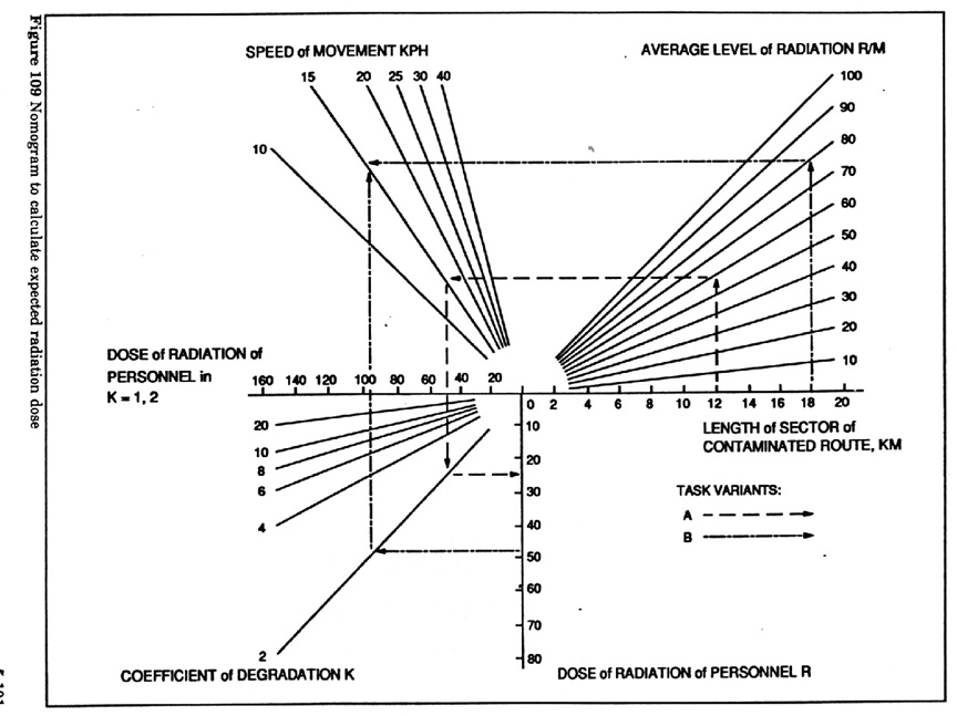
|
|
| |
(26) Calculation to Select the Optimal Travel
Route
This is an extremely important and varied class of calculation. The example
given here is only illustrative of the possibilities for employing the given
method for solving problems of optimization from among a small set of possible
variants.
The commander of a sub-unit has a mission to break out to an assigned line and
assume the defense in the shortest possible time. There are five possible
travel routes to reach the assigned position. All routes pass through a zone of
radioactive contamination. Therefore, an additional condition of the advance is
the expected dose of radiation received by sub-unit personnel. It is apparent
that in this example there are five decision variants. The main criterion for
evaluating their relative effectiveness is the travel time. The shorter the
better. However, the commander must also strive to keep the received radiation
dose at a minimum, or at least not allow it to exceed a set maximum per norms,
for instance 05 roentgens.
The conditions for the sub-unit to advance to the assigned mission line may be
expressed in a table showing quantitative characteristics. From the data it
becomes obvious that the possible movement routes differ from each other in
length, road quality, and mean level of radiation.
From the table we see that on route 1 in advance variant 1 there are four
segments of 16 km of highway, )travel speed 40 km/hr( 10 km of improved dirt
road )travel speed 25 km/hr(, 9 km of dirt road )travel speed of 15 km/hr (,
and 5 km of damaged, nearly impassable road )travel speed > 5 km/hr(. The
mean radiation level on the entire first route is 100 roentgens per hr. From
this information we can calculate the expected duration of travel time to reach
the mission line, as follows:
t1=)16 ÷ 40( + )10 ÷ 25( + )9 ÷ 15( + )5 ÷
5(=2.4 hrs or 2 hrs, 24 min. The first route passes through a radiation zone of
100 roentgens per hr. Using the previous method for calculating radiation with
a reduction factor of K=4 for equipment D=) 100( )2.4( ÷ 4=60 roentgens.
After calculating the same data for the other four routes the information
needed for the decision may be shown in another table of movement time and
expected radiation dose.
|
|
| |
Figure 110 Table to enter description of travel routes
|
QUANTITATIVE CHARACTERISTICS OF ALTERNATE ROUTES
|
| Advance route number |
Length, km, of route segments of different
road quality |
Mean radiation level on route,
R/hr |
| 1st |
2nd |
3rd |
4th |
| 1 |
16 |
10 |
9 |
5 |
100 |
| 2 |
-- |
20 |
12 |
4 |
120 |
| 3 |
29 |
12 |
6 |
2 |
120 |
| 4 |
-- |
15 |
20 |
5 |
60 |
| 5 |
16 |
15 |
3 |
4 |
80 |
| Travel speed along each segment km/hr |
40 |
25 |
15 |
5 |
|
|
|
| |
Figure 111 Graph of effectiveness of
alternate routes
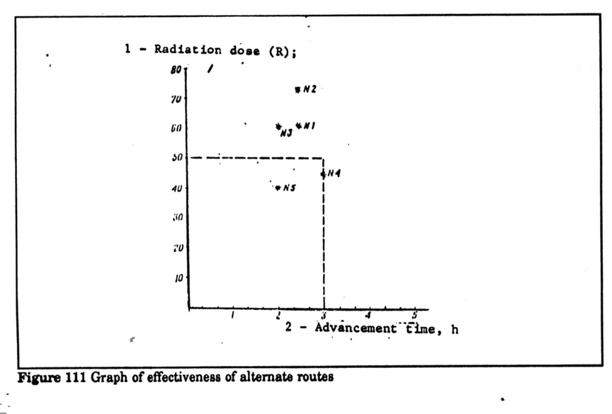
|
|
| |
Figure 112 Table of effectieness indicators
for march routes
| EFFECTIVENESS INDICATORS FOR
TRAVEL ON VARIOUS ROUTES |
| Route )variant( number |
Time to move forward )hr( |
Expected radiation dose, R |
| 1 |
2.4 |
60 |
| 2 |
2.4 |
72 |
| 3 |
2 |
60 |
| 4 |
3 |
45 |
| 5 |
2 |
40 |
|
|
| |
These results may now be compared to determine the optimum
decision of which route to choose. Displaying this data in the table makes it
easy to see that the optimum solution is route number 5, having both the
shortest travel time and lowest radiation dosage, however this might not always
be the case. We can also see that the shortest route )no 2( is actually worse
than the longest ) no 3(. However, a more general technique for solution, when
the answer is not evident is to prepare a graph to plot the information. In
this example plot the radiation dose on the y axis and the travel time on the x
axis. Then enter the coordinates for the given mission requirements, such as
maximum travel time of 3 hrs and maximum radiation dose of 50 roentgens. Draw
vertical and horizontal lines from the axes to the selected coordinates. Plot
the data for all the possible variants. Those variants whose position falls
within the rectangle formed by the axes and the lines to the decision point.
|
|
| |
(27) Calculation to Determine Optimal Distribution
of Weapons
One of the most important classes od decision for the commander is the optimal
distribution of weapons against various targets. This is a more complex
calculation that the previous example of optimum route given two decision
criteria. As an example consider the distribution of weapons against a group of
targets. The calculation technique shows the course and result of the
calculation for optimization. Of course, the ideal solution technique is to use
computers, and Soviet headquarters are certainly using this method. In the
field, however, the commander may be required to make a rough calculation
without having a computer available. The following simple method produces
sufficiently reliable results when a small number of forces and means and
targets are being considered. The illustration, nevertheless, indicates the
type of problem for which computer solutions may be developed.
In this example the commander must find the most effective distribution of five
different groups of weapons against five strong points in order to inflict the
maximum casualties on the enemy. having calculated the effectiveness of fire of
each of the groups of weapons against each target, for instance, using the
technique with the nomogram ) ( the commander may create a table of
effectiveness of damage to each enemy target by each weapon.
|
|
| |
Figure 113 Table of effectiveness of artillery fire on
targets
| EFFECTIVENESS OF ARTILLERY
FIRE DAMAGE ON TARGETS |
| Weapons group |
Damage effectiveness in
hectares for target number |
| 1 |
2 |
3 |
4 |
5 |
| 1 |
3 |
4 |
3 |
5 |
9 |
| 2 |
4 |
7 |
5 |
4 |
7 |
| 3 |
6 |
8 |
3 |
5 |
9 |
| 4 |
2 |
6 |
9 |
8 |
5 |
| 5 |
9 |
4 |
2 |
2 |
4 |
|
|
| |
The damage achieved by different weapons against various
types of targets is not identical because of the difference in the quantity and
quality of the weapons, the quality of the shells, and the relationship of the
ballistic characteristics of the weapons )dispersion pattern etc( to the
dimensions of the targets, and the degree of shelter of the enemy personnel.
According to the data in the table, the first group of weapons when hitting the
first enemy target inflicts casualties to the personnel in an area of 8
hectares, the second weapons group against the same target damages 4 hectares,
and so on.
If the commander assigns the first weapons group against the first target, the
second group to the second target, etc., then the effectiveness of the
distribution will be the total area damaged or 03 hectares. However, this
solution will not be optimal, since the actual combat capabilities of the
available weapons in these conditions are not used in the best way. In order to
find the best distribution and solve the problem quickly, another method for
calculation must be used. The initial data for this are shown in the next
table; the weapons groups, the number of target groups and the firing
effectiveness.
The calculation of the optimal distribution is performed directly on the table.
First, select the two greatest values for the effectiveness values in each
line. In the first line these are 9 and 8, and in the second they are 7 and 7,
etc. Then subtract the lesser value from the greater and write the results in
the right hand column, as shown. Perform the calculation first by each line and
then by each column. Examine the differences by lines and columns, select the
greatest value and mark it )*(. In this example the result is the fifth line,
but the maximum may also be in a column. Then in the line or column in the
fields for which the greatest value shows, find the maximum indicator and
underline it. )This is the 9 in line 5 column 1.( This indicates that the fifth
weapons group should be targeted against the first target group. Eliminate this
pair from further consideration.
The course of the further calculation is shown in the next table. The remaining
weapons are in a similar manner distributed against the remaining target groups
until all groups of weapons are distributed.. This shows that the first group
should fire on the fourth target, the second on the second, the third against
the fifth, and the fourth against the third. This results in the greatest
damage to enemy personnel, a total area of 42 hectares. This is the maximum
value of damage from the 120 possible combinations of weapons and targets in
the example.
|
|
| |
Figure 114 Table of effectiveness of artillery fire on
targets
| EFFECTIVENESS OF ARTILLERY
FIRE DAMAGE ON TARGETS )COURSE I( |
Course 1 |
| Weapons group |
Damage effectiveness in
hectares for target number |
| 1 |
2 |
3 |
4 |
5 |
| 1 |
8 |
4 |
3 |
5 |
9 |
1 )9-8( |
| 2 |
4 |
7 |
5 |
4 |
7 |
0 )7-7( |
| 3 |
6 |
8 |
3 |
5 |
9 |
1 )9-8( |
| 4 |
2 |
6 |
9 |
8 |
5 |
1 )9-8( |
| 5 |
9 |
4 |
2 |
2 |
4 |
5* )9-4( |
| C-1 |
1 )9-8( |
1 )8-7) |
4 )9-5( |
0 )8-8( |
0 )9-9( |
|
|
|
| |
Figure 115 Table of effectiveness of artilleyr fire on
targets
| EFFECTIVENESS OF ARTILLERY
FIRE DAMAGE ON TARGETS )COURSE I( |
Course 1 |
C 2 |
C 3 |
C 4 |
| Weapons group |
Damage effectiveness in
hectares for target number |
| 1 |
2 |
3 |
4 |
5 |
| 1 |
8 |
4 |
3 |
5 |
9 |
1 )9-8( |
1 |
1 |
- |
| 2 |
4 |
7 |
5 |
4 |
7 |
0 )7-7( |
0 |
0 |
0 |
| 3 |
6 |
8 |
3 |
5 |
9 |
1 )9-8( |
1 |
1 |
1 |
| 4 |
2 |
6 |
9 |
8 |
5 |
1 )9-8( |
1 |
- |
- |
| 5 |
9 |
4 |
2 |
2 |
4 |
5* )9-4( |
- |
- |
- |
| C-1 |
1 )9-8( |
1 )8-7) |
4 )9-5( |
0 )8-8( |
0 )9-9( |
|
|
|
|
| C-2 |
- |
1 |
4* |
0 |
0 |
|
|
|
| C-3 |
- |
1 |
- |
3* |
0 |
|
| C-4 |
- |
1 |
- |
- |
2* |
|
In this example the total area of damage was considered the indicator of
effectiveness. Sometimes one must minimize the effectiveness indicator instead
of maximizing it. For instance, the indicator might be the time required for
fulfilling the mission, the expenditure of munitions or other materials, etc.
Top optimize the distribution according to a minimum indicator value, use the
same technique, only in calculating the differences in the lines and columns,
select two minimum values instead of the two maximum ones and subtract the
least from the greatest. Then find the minimum indicator in the appropriate
line or column and fix it first.
This comparatively simple and practical technique for determining the optimum
distribution of forces and means is useable in the field. The materials being
distributed might be weapons, reconnaissance means, communications systems,
water crossing equipment, etc.
|
|
| |
(29) Calculation to Determine the Effectiveness of
Fire Destruction Means
This is a more elaborate version of the basic formula designed for use with
calculators. The initial data is the number of fire targets, the number of
weapons, rate of fire, and coefficient of effectiveness of fire, the length of
time for conducting fire, and the coefficient of resistance )counteraction( of
the enemy. The formula is:
where:
M=quantity of targets to be destroyed;
Nt=total number of targets;
Pi=probability of destruction of target from one weapon by one shot;
q=probability of destruction of weapon by fire of enemy;
Nw=number of weapons;
=rate of fire )number of rounds per min(;
t=duration of fire in min.
Example problem: Determine the expected number of destroyed targets from 30
observed targets, if 12 weapons with a rate of fire of 3 rounds a minute are
used for their destruction. The probability of destruction by 1 shot is 0.2 and
firing time is 5 min. The probability of destruction of our weapon by enemy in
the time of one shot is .3
|
|
| |
Figure 116 Form for calculating weapons effectiveness
|
FORM FOR CALCULATING WEAPONS EFFECTIVENESS CONSIDERING ENEMY
COUNTERMEASURES
|
| No |
Initial data and values to be
determined |
Units |
Calculation variant |
Remarks |
| Example |
2 |
3 |
| 1 |
Number of targets |
units |
30 |
|
|
|
| 2 |
Probability of destruction in one shot |
-- |
0.2 |
|
|
|
| 3 |
Probability of destruction by enemy during one shot |
-- |
0.3 |
|
|
|
| 4 |
Number of weapons |
units |
12 |
|
|
|
| 5 |
Firing rate |
rounds / min |
3 |
|
|
|
| 6 |
Firing time |
min |
5 |
|
|
|
| 7 |
Number of destroyed targets |
units |
18 |
|
|
|
|
|
| |
Reconnaissance Planning
Reconnaissance planning makes use of many of the same calculations and formulas
used for operational planning, such as time and distance for movements and
optimization of resources. The following are some calculations specifically
designed for reconnaissance planning.
30) Calculation of Effectiveness of Reconnaissance and Required
Duration for a Reconnaissance Mission
The given data for the calculation is the speed of movement of the
reconnaissance means, the actual range of observation of reconnaissance, the
dimensions of the area being covered and the duration of the patrol. The
formula is:

|
|
| |
P=probability of observing an object )target(;
e=natural logarithm 2.72;
R=radius of observation of targets by reconnaissance in km;
V=rate of movement of reconnaissance means during the mission in km/hr;
t=duration of patrol;
S=area of the region being observed in sq km.
If it is required to observe several targets in one area, then the mathematical
expectation of coverage )average number of targets seen( for observed targets
can be calculated as M=N x P
where M=average number of observed targets; N=total number of targets in the
area;
and R=probability of detection of one target.
To determine the duration of patrol in order to observe a target with a
pre-determined likelihood for observation the formula is:

Example problem: Determine the likelihood of observation of targets after 2
hours of reconnaissance in an area of 58 sq km if the effective observation
distance is 1.5 km and rate of movement of the patrol is 12 kph. The table
shows the answer that the probability of observation coefficient is .71. Answer
is that if there are 15 targets in the area then they can find 10 to 11 of
them.
|
|
| |
Figure 117 Form for calculating probability of target
detection
FORM FOR CALCULATING
PROBABILITY OF DETECTING TARGETS
|
| No |
Initial data and values to be
determined |
Units |
Calculation variant |
Remarks |
| Example |
2 |
3 |
| 1 |
Effective target detection range |
km |
1.5 |
|
|
|
| 2 |
Reconnaissance system speed |
km/hr |
12 |
|
|
|
| 3 |
Search duration |
hr |
2 |
|
|
|
| 4 |
Search region area |
sq km |
56 |
|
|
|
| 5 |
Target detection probability |
-- |
0.71 |
|
|
|
Example problem 2: Determine the duration of time to perform the
reconnaissance mission to observe a target in an area of 50 sq km to a
likelihood percentage of 80%, if observation distance is 1.2 km and rate of
movement is 15 kph. Answer is 4.5 hr
|
|
| |
Figure 118 Form for calculating length of
search
|
FORM FOR CALCULATING LENGTH OF RECONNAISSANCE SEARCH
|
| No |
Initial data and values to be
determined |
Units |
Calculation variant |
Remarks |
| Example |
2 |
3 |
| 1 |
Target detection probability |
-- |
0.8 |
|
|
|
| 2 |
Search region area |
sq km |
50 |
|
|
|
| 3 |
Effective target detection range |
km |
1.2 |
|
|
|
| 4 |
Reconnaissance system speed |
km/hr |
15 |
|
|
|
| 5 |
Search duration |
hr |
4.47 |
|
|
|
|
|
| |
(31) Calculation of Detection of Targets by
Reconnaissance
If the probability of detection of targets at a given range may be considered
as approaching 1, then the formula for calculating the probability of detecting
a target in an area during a patrol of given length can be simplified to
eliminate the logarithm. The simplified formula may in turn be structured into
a nomogram for even faster calculations. In this case the initial data for the
calculation are the length and speed of the search, and the range of reliable
target detection ) probability near 1.0( of the reconnaissance systems. The
formula is:

where:
2RVt is less than or equal to S;
P=probability of target detection;
R=effective range of reliable observation in km;
V=search speed in km per hr;
t=search time in hours;
S=surface area of the search region in square km.
Example calculation using formula: Determine the probability of target
detection in 2.5 hours in an area of 37 sq km when the search speed is 4 km/hr.
Solution is P=}2 x 1.3 x 4 x 2.5{ ÷ 37=0.7
|
|
| |
Example calculation using the nomogram Figure 119:
Determine the probability of detection of a target in 3 hrs in an area of 50 sq
km, when the range of detection is 1.2 km and the search speed is 6 km/hr.
Solution: For this calculation )variant a( draw a perpendicular line from the
"1.200" mark on the "Reliable detection range" scale to the
intersection with the "Search speed - 6" line. From the point draw a
horizontal line to the right to intersect the "Search length - 3"
line, then from this point draw a horizontal line to the left to the
"Probability of detection" scale. Read the answer at 0.86.
Example 2: Determine the search length in an area of 60 sq km, when the target
detection probability is 0.9, the reliable detection range is 1.3 km and the
search speed is 8 km/hr.
Solution: For this calculation )variant b( draw a horizontal line to the right
from the "0.9" mark on the "Probability of detection" scale
to the intersection with the "Search region area - 60" line. From
this point draw a vertical line. Then draw a perpendicular line from the
"1.300" mark on the "Reliable detection range" scale to the
intersection with the "Search speed - 8" line. From this point draw a
horizontal line to the right to the intersection with the previously draw
vertical line. They intersect along the "Search length - 2.5" line.
The answer then is approximately 2.5 hours required to complete the assigned
search.
|
|
| |
Figure 119 Nomogram for calculating
probability of target detection

|
|
| |
Sample Calculations for Division and Army
Staff
|
|
| |
Example calculation using formulas: On the basis of army's
initial instruction the division staff calculates the time its lead regiment
requires to move to the border area and deploy there when:
depth of regiment column - 30 km
depth of the area of deployment - 6 km
average speed of march - 20 km
distance to the border area - 120 km
Solution: Use the formula:
where
t=time the regiment needs to deploy in new area
D=distance to border area
V=average speed of march
GK=depth of regiment column
GR=depth of the area of deployment
tp=time spent for halts
t=(120 ÷ 20) ( + (30 - 6) ÷ (0.6 x 20) + 1=9 hrs
Example calculation: On the basis of the same instructions the division
determines the time for the division to deploy and occupy the designated
departure area when:
- depth of division columns on 3 routes - 80 km
- depth of the area of deployment - 35 km
- average speed of march - 25 km
- distance to departure area from start line - 125 km
- time to complete engineer work - 8 hours
Solution: To solve the problem the staff applies a combination
of calculations and norms. Calculations are done both in general terms )time to
complete the deployment for the entire division( and calculations to determine
the time of deployment of different echelons such as first and second echelons,
rear service troops, air defense troops, attack helicopters etc. The method is
the same for all categories. In each case normatives are applied to determine
the time required for specific tasks such as engineer work, establishment of
fire system, delivery of supplies, loading and unloading, establishment of
security, etc.
A. Calculations in general terms:
T=)D ÷ V( + tp + )Gk - GR( ÷ 0.6V +
tengr
T=125 ÷ 25 + 1 hr + )80 - 35( ÷ )0.06 x 25( + 8 hrs
T=5 + 1 + 3 + 8=17 hrs.
B. Calculations in specific terms
1. For the first echelon regiments )depth of column 30 km, depth of area of
deployment 10 km(:
T=(150 ÷ 25) + 1 + (30 - 10) ÷ (0.6 x 25) + 8 hrs ....(1)
T=6 + 1=1:20 + 8 hrs=16:20 hrs
2. For second echelon regiments use the same formula:
T=170 ÷ 25 + 1 + (30 - 11) ÷ (0.6 x 25) + 8 .....(2)
T=6:48 + 1 + 1:20 + 8=17.08
3. For the rear service use the same formula:
T=195 ÷ 25 + 1 + (10 - 5) ÷ (0.6 x 25) + 8 ......(3)
T=7:48 + 1 + 0.20 + 8=17:08
|
|
| |
Notes: )1( Movement distance for first
echelon regiments is assured to be 150 km on the basis that the regiments
should move another 25 km from the division deployment line to reach there
designated position in the first echelon 125 + 25=150
)2( The distance for the second echelon is assumed to be 0`7 km on the basis
that the regiment moves 35 km from the head of the column )depth of first
echelon regiment plus 5 km interval( and to reach its designated area it should
move another 01 km from the divisions to reach its area of deployment in the
second echelon (125 + 35 + 10=170 km)
)3( The distance for the rear service is assumed to be 195 km to include its
distance from the head of the column )65 km( and the 5 km interval ) 125 + 65 +
5=195 km(
Example problem: The division commander must clarify his
mission and calculate the following on the basis of the army commander's
instructions.
- depth and width of the division missions;
- width of the area of penetration;
- required rate of advance;
- number of regiments required in first and second echelon.
Solution:
1. The depth and width of the division mission is measured on the map in the
following manner:
- depth of the immediate mission 17 km with a width of 8 km
- depth of long range mission is 21 km and a width of 12 km
- the width of penetration area is 3.5 km, requiring the forces and means of
two regiments )2 km and 1.5 km of penetration area assigned to them(, the
remaining 4.5 km of the front should be covered by part of one of the regiments
of the penetration area )the right flank regiment( and forces and means of
another regiments.
2. The immediate mission to be accomplished in ------- hours )assume 7 hours(
therefore the average rate of advance is 17 ÷ 7=2.5 km/h. The long range
mission is to be accomplished in ------ hours )assume 5 hours(, therefore the
average rate of advance should be 21 ÷ 5=4 km/h
3. On the basis of the width of penetration area which is 3.5 km )the norm is 2
km per regiment( and the overall width of the division sector i.e. 8 km there
can be two alternatives for the echelonment of the troops:
a. Two regiments in the first echelon, one BMP regiment covering the
front and one regiment in the second echelon to be committed after the
penetration of the enemy's brigade defensive position, while the BMP regiment
will then constitute the second echelon to be committed after the penetration
of enemy's division defenses.
b. Three regiments in first echelon, with the BMP regiment coming to the second
echelon after the attack is begun.
4. Therefore the commander can tentatively determine the following:
- rate of advance
- direction of the main attack and the width of penetration area
- combat formation of the division for the attack
5. Issues mentioned in point 4 are further examined , elaborated and confirmed
during the estimate of the situation and "recognasirovka".
Example problem: As the chief of operation section prepare for
the commander calculations to determine the required correlation of forces and
means to support the assigned rate of advance.
Solution: To solve the problem use the rate of advance
nomogram. To use the nomogram first find the F factor
F factor=D ÷ KTVmax;
D=distance )depth( of the mission
K=terrain coefficient:
-- 1.25 level
--1.00 rough-level
--.75 rugged hills
--.75 urban sprawl
--.50 mountainous
T=time required for action in days and fraction of days
Vmax=theoretical speed in km/day
F=38 ÷ (1.25 x 1 x 60 )=0.5
Now see in the nomogram what correlation of forces and means is required when
the F factor is 0.5 The answer is 4.3:1
Example problem: Determine the width of the main sector on the
basis of the following facts:
- width of the overall area of the division is 8 km
- overall correlation of forces and means is 3: 1
- required correlation of forces in the main sector is 4.3:1
- correlation of forces and means below which we can not drop in the rest of
the division area is 2:1
Solution: Use the size of the sectors formula which is as
follows:

Wm=width of the main sector
Wo=width of the overall area
Co=overall correlation of force
Cm=required correlation of force
Cs=correlation of force below which one can not drop in the rest of
the action area.
Wm=8 (3 - 2) ÷ (4.3 - 2)=3.5 km
Note: You can increase the width of the main sector area by
accepting a lower correlation of forces and means in the rest of the area of
division attack, for example:
Wm =8 (3 - 1.3) ÷ (4.3 - 1.3)=13.6 ÷ 3=4.5 km
Example problem: Calculate the time for a division to advance
from the assembly area )departure area( and deploy for shift into attack from
the line of march when:
- distance of attack line from enemy forward line=1 km:
- distance of line to deploy into company column=4 km:
-distance of line to deploy into battalion column=12 km:
-distance of regulating line to line of deployment into battalion column=20 km:
- distance of regulating line from start line=40 km:
- distance of start line from assembly area=5 km:
- depth of first echelon regiments=30 km:
- interval between 1st and 2nd echelon regiments=10 km:
- movement speed into attack=8 km:
average speed during march=24 km/h:
Solution: This calculation can be done either by using several formulas to
calculate each section of the advance and finally to combine them together or
by filling in prepared tables.
a. Using formulas: 06 should be 60 and 09 should be 90:


ta=time for crossing final deployment into line of attack minus
)H( in minutes:
Da=distance of line for going into attack formation from the forward
edge of the enemy position in km:
Va=rate of movement in attack formation in km/h:
tr=time for crossing the line of deployment into company column )H
-minutes(:
Dr=distance of line of deployment into company columns from the line
of deployment into attack formation in km:
v=average rate of movement of units in mounted formation during march:
tb=time for crossing line of deployment into battalion column )H
-minutes(:
Db=distance of line of deployment into battalion columns from line
of deployment into company columns in km:
trr=time for crossing the last regulation line )LRL( prior to
deployment into battalion columns )BC(:
Drr=distance of LRL to BC:
ti=time for passing the start line )SL(:
Di=distance of SL from LRL:
tvit=time to begin movement from assembly area
D=distance of SL from assembly area:
ti'=time for crossing the SL by second echelon:
Gk=depth of the mounted column of first echelon in km:
Dk=distance between the tail of the first echelon and the head of
the second echelon in km:
60 and 90=coefficient for conversion of time in minutes for the average speed
during the deployment on each line:
ta=)1 x 60 ÷ 8=7.5 ) H - 7.5 min(
tr=7.5 + )4 x 90( ÷ 24=7.5 + 15 min=)H - 22.5 min(
tb=22.5 + )12 x 60 ÷ 24=22.5 + 30 min=)H - 53 min(
trr=52.5 + )20 x 60 ( ÷ 24=25.5 + 50=)H - 1hr,43 min(
ti=01:43 + )40 x 60( ÷ 24=01:43 + 01:40=)H - 03:23(
tvit=03:23 + )5 x 99( ÷ 24=03:23 + 00:19=)H - 03:42(
ti'=03:42 + )30 + 11( x 90 ÷ 24=03:42 + 02:30=) H -
06:12
b. Using the tables:
The same calculations can be done by using the tables given above with the
individual calculations and filling in the numbers in each line. Such tables
are pre-prepared in advance in blanks and the operation staff can use them to
do calculations taking different options into consideration.
Sample calculations: Determine the time and distance to the line of meeting
with a counter-attacking enemy reserve when:
- the enemy reserve )up to 2 mech and 2 tank battalions( is sighted 28 km from
the forward line of division's attacking troops:
- enemy's speed of advance is about 15 km/hr:
- a delay of 30 minutes is expected in the enemy movement due to a narrow area
along the road:
- planned air strikes and artillery fire's are expected to delay the enemy for
another 40 minutes:
- the speed of own attacking forces in the first echelon is 4 km/hr due to
isolated enemy's strong points across the front:
- the attack on enemy's position 4 km further in the depth )the troops are
expected to reach there within an hour( is expected to delay 45 minutes for
minor regroupment.
|
|
| |
Solution: use the formula:

tv=expected time of meeting the enemy in hours:
D=distance between opposing forces in km
tn=total delay time for own forces in hours
Vn=speed of movement of own forces
tp=total delay time for enemy forces
Vp=speed of movement of enemy forces
Results:
tv=}28 + ])0.75 x 4( + )1.15 x 15 ([{ ÷ )4 + 15(
tv=]28 + )3 + 17.35({ ÷ 19
tv=)28 + 02.25( ÷ 19 : tv=2.54 or 2 hrs and 33
minutes
Now to determine the distance of meeting with the enemy use this formula:
lp=Vn )tv - tn (
lp=4 )2.54 - 0.75(
lp=7.16 km
This means that the first echelon forces will be able to destroy the enemy in
this intermediate defensive position before it can launch its counter-attack,
provided the enemy's reserve is delayed by air strikes and artillery fire for
not less than 40 minutes and the enemy does have to slow down 30 minutes delay
to cross the narrow pass and own forces do not take more than 45 minutes to
regroup in order to continue the attack. If the division commander determines
that the line of meeting with the enemy is not convenient, he can chose to
repel the counter-attack from a line further in back or he might want to
further delay the enemy so that the first echelon troops can move further than
7.16 km before the enemy launches his counter-attack. This calculation can also
be conducted by filling in the pre-prepared form.
Example calculation: On the basis of the assumptions which were mentioned in
exercise 01 determine the number of anti-tank weapons )ATGM and AT guns( to
repel the enemy tanks when:
- the number of enemy tanks are estimated to be 80:
- no less than 50% of enemy tanks must be destroyed:
- the probability of destruction of a single tank by one weapon with one shot
is 0.2:
-up to 8 rounds may be fired by each weapon in the time the tanks are located
in the effective zone of fire:
Solution: To determine the required number of anti-tank
weapons use the formulas or the nomogram.
Formulas:


Mn=degree of destruction of tanks by artillery )in percentage(;
P1=probability of destruction by one weapon in one shot;
N=required number of anti-tank weapons to accomplish the mission;
m=weapon rate of fire or number of shots one weapon can shoot during the time
the target is in within range;
M=expected number of attacking tanks.
This method is a lengthy one and difficult to use under field conditions.
The nomogram can be used for up to 40 tanks. However, for over 40 tanks divide
the number into pieces less than 40 and calculate on the basis of the nomogram
and add the results: 60=40 + 20, or 77=40 + 37 etc.
In this example the following calculation can be done on the nomogram: Draw a
perpendicular line from 0.5 mark on the "Required amount of destruction of
targets" scale to intersect with the "Probability of target
destruction by one round 0.2" curve. From this point draw a horizontal
line to the intersection with the "Number of attacking ground targets -
40" line and then a vertical line up to the "Number of firing by one
weapon - 8" line. From this point go along the horizontal to
"Required number of antitank weapons" scale and read 17 then multiply
it by 2 to get the required number of AT weapons for 80 tanks: 17 x 2=34 AT
weapons.
Example calculation: The division commander decided to use the divisional AT
reserve at the line for repulsing the enemy's counter-attack, which previous
exercise set at 7 km up from the current forward line of the first echelon
troops. The AT reserve is now 8 km from the forward line. The enemy is 12 km
away from the line of repulsion of counter-attack with an expected delay of 1
hour and 10 minutes on the way )due to planned air strikes and artillery's
fire(. The speed of advance of the enemy is 15 km/hr the effective range of AT
weapons is 3 km. The AT reserve will need 30 minutes to deploy on the fire line
and prepare for action. It's speed of movement 12 km/hr.
|
|
| |
Determine how much time is available for the division
commander and staff to assign mission to the AT reserve.
Solution: Use the formula:

where:
t=time available for the commander and his staff to assign mission;
D=distance of the enemy to the line of contact;
tp=total delay time for enemy forces;
Vp=speed of movement of enemy forces;
d=effective range of AT weapons;
tn=total time required for AT reserve to move to the line of the
repulsion of the enemy's counter-attack and time to prepare for action.
1. First determine the tn
 : :
tn=time for AT reserve to move and prepare for action;
Vn=speed of movement of AT reserve;
tr=time to prepare for action;
tn=)8 + 7( ÷ 21 + 0.5=1.57.
2. Now determine the t:
t=}]D + )tp x Vp([ - d{ ÷ Vp -
tn
t=}]21 + )1.15 x 15 ([ 2{ ÷ 15 - 1.75
t=])21 + 17.5( - 2[ ÷ 15 - 1.75
t=)38 - 2( ÷ 15 - 1.75
t=36 ÷ 15 - 1.75
t=2.25 - 1.75=0.5
t=30 minutes.
This means that the division commander and staff should assign mission to the
AT reserve within 30 minutes )not later( so that the AT reserve will arrive and
get prepared on the line of repulsion before the enemy tanks reach the
effective range of AT weapons at the line.
Example calculation: In planning the commitment of divisions's second echelon
the area within 4 km of the enemy intermediate defensive position, which is to
be attacked by the second-echelon, is open and when the regiment moves and
deploys to company and platoon columns and assumes the combat formation in this
area, it should be covered by artillery strikes conducted on enemy strong
points at the line of commitment and on the flanks. The line of attack is 1 km
and the line of fire safety is 400 m from enemy position. The speed of movement
is 20 km/hr and speed of attack is 6 km/hr. Determine the duration of artillery
strike to cover the deployment and attack of the second-echelon regiment.
Solution: To determine the duration of artillery strike
calculate the time it takes the regiment to deploy and move to the line of
attack and then to the safety line of fire in front of enemy position (400 m).
Use equations:
t=ta + tr ...........)1(


t=time of artillery strike;
ta=time for crossing the attack line up to the fire safety line;
tr=time spent from deployment in the company columns up to the line
of attack;
Da=distance of attack line from enemy position;
d=distance of fire safety line to the enemy position;
Va=speed of movement in attack;
Dr=distance of deployment into company columns;
V=speed of movement of troops;
Results:
ta=)1 -0.4( x 60 ÷ 6=6 minutes
tr=3 x 90 ÷ 20=27 ÷ 2=13.5 minutes
t=ta + tr=6 + 13.5 approximately 20 minutes
This means that the artillery strike should be conducted for 20 minutes to
cover the commitment of the second echelon regiment.
Example calculation: The division has accomplished its immediate mission and
continues the attack in depth to complete the destruction of the enemy forces
in its tactical zone and accomplish the long range mission by the end of the
day. The first echelon regiments are fighting with the enemy forces, which
conduct delaying action and cover the withdrawal of its main forces across the
Schmalin River. Two enemy battalion size columns 15 km from the river are
withdrawing to the river apparently to establish defense on the river. The
division commander has decided to assign a forward detachment to prevent the
arrival of these enemy battalions on the river. The distance to the enemy
columns from the head of the assigned forward detachment is 15 km. A 20 minute
delay is expected in the movement of enemy columns due to planned friendly air
strikes. The speed of movement of enemy's columns is 15 km/hr.
Determine the expected time and rate of overtaking of the withdrawing enemy by
division's forward detachment.
Solution: Here the crucial issue is to overtake the enemy
before he is able to cross and establish defense at the river.
1. First determine how long does it take the enemy to reach the river:
t=D + )tp x Vp( ÷ Vp
t=time it takes the enemy to reach the river;
D=distance of the enemy to the river;
tp=expected delay in enemy's movement;
Vp=speed of enemy's movement;
Results:
t=]15 + )0.5 x 15 ([ ÷ 15
t=(15 + 7.5) ÷ 15=22.5 ÷ 15=1.5
t=1 hr and 30 minutes
Therefore the enemy's columns must be overtaken within less than 1.5 hours.
2. Assume that the speed of movement of the forward detachment is 20 km/hr:
Now to=]D - )tp x Vp ([ ÷ )Vn
- Vp (
to=time to overtake the enemy )hours(;
D=distance to the enemy;
tp and Vp=same as in 1;
Vn=speed of movement of own forces )forward detachment(;
to=15 - (0.5 x 15) ÷ (02 - 15)
to=)15 - 7.5 ) ÷ 5
to=7.5 ÷ 5=1.5
to=1 hour and 30 minutes
This means that at a speed of 20 km/hr the forward detachment can not catch the
enemy columns before they reach the river. In order to overcome this, either
the speed of movement should be increased or the enemy should be further
delayed by air strikes, airborne assault troop, artillery fires, mines etc.
3. In order to find the required speed of movement of the forward detachment to
overtake the enemy in one hour perform the following calculation, using the
formulas:
Vn=}]D - tp x Vp([ + )to x
Vp({ ÷ to
Vn=]15 - )0.5 x 15 ([ + ])1 x 15 ([ ÷ 1
Vn=(7.5 + 15 ) ÷ 1=22.5 ÷ 1=22.5
Vn=22.5 km/hr.
Therefore the speed of movement of the forward detachment should be at least
22.5 km per hour to ensure the enemy's interception within an hour. At that
time the enemy will be 7.5 km from the river.
D=)t x Vp( - )tp x Vp(
D=)1 + 15( - )0.5 x 15(
D=15 - 7.5=7.5 km
|
|
| |
Calculations for Front Offensive
Planning
One of the most important preliminary calculations made by the front
commander is for the allocation of his forces to first and second-echelons and
to main and secondary attack axes )directions(. This is done on the basis of
the correlations of forces required to achieve assigned results in the attack
sectors and the minimum correlations allowable in other )holding attack(
sectors. In addition the quantity of artillery available to meet density norms
will also be a governing factor.
Example calculation: Presume the initial instructions received by the
front commander establish the following: the front is
assigned a mission for offensive operation with the scope:
- overall depth: 640 km
- depth of immediate mission: 280 km
- depth of long range mission: 360 km
- width of the frontage: 340 km
- duration of operations 14 days
The front is composed of four combined arms armies on D day, a tank
army will join the front on D + 2.
During the clarification of the mission the commander determines the following:
- number of attack directions and breakthrough areas;
- number of armies in the first echelon;
- rate of advance, and required correlation of forces for such rate of advance.
Answer:
Since the direction of the main attack is determined by the superior commander,
the front will facilitate the establishment of the appropriate
grouping of forces and means and support of the axis. In this case the
front also has a choice to determine the number of supporting attacks
and forces allocated to them.
1. On the basis of initial data the front has one direction of main
attack. According to theory a major part of the forces should be allocated to
this direction: two armies with a frontage of not more than 60 km in a European
type of terrain ) 60 x 2=120 km of front). Now what is left is 340 - 120=220
km. Therefore this 220 km is to be covered by two more armies.
If the front launches a supporting attack with one army, it cannot
give the army a sector of more than 08 km.
)therefore: 220 - 88=140 km(.
Now if one army is assigned this 140 km front, it cannot attack; but only will
hold the line or it may attack in a narrow sector merely to support the main
attack of the supporting attack directions.
These are preliminary deductions based on the clarification of the mission.
These variants can be further developed during the estimate of the situation.
The determination of the number and overall width of the breakthrough areas
depends on the number of armies and divisions in the first echelon. This is
again a tentative and rough assessment, while the more detailed calculation can
be conducted later, on the basis of artillery capability and number and type of
enemy targets.
Penetration areas:
- main direction: 2 armies each 12 km=24 km
- supporting direction: 1 army 10 km - 10=total of 34 km
2. Rate of advance:
a. 640 ÷ 14=45 km/day
This is the average rate of daily advance which should be maintained. In order
to see if this rate of advance can be maintained, make an overall and summary
correlation of forces and means. A 3:1 correlation supports an average rate of
advance of 40 to 60 km/day.
b. To find out the required correlation of forces and means )basically on the
main direction( use the formula/nomogram of )"Correlation of forces needed
for rates of advance"(:
f )factor(=D ÷ KTVmax;
f=correlation factor;
k=terrain factor )1.25 for open terrain(;
Vmax=theoretical speed in km/day.
On the nomogram read that a correlation of 4.6 to 1 is required to achieve the
accomplishment of the mission in 14 days. This is a rough calculation and the
enemy's detailed capabilities are not taken into consideration. This
correlation mostly applies to the axes of main attack, while on axes with
holding attacks a lower correlation can be accepted.
Assume that the four divisions attacking in the right flank army and the three
divisions attacking in the army adjacent to it to the south are the main
direction.
On the supporting direction three divisions of the left flank army attack in
the first-echelon with one division of the adjacent army to the north
participating in the breakthrough. Determine the overall breakthrough area and
number of artillery pieces required.
Answer:
1. Main direction: 4 divisions + 3 divisions=7 divisions: the norm for the
width of the breakthrough area per division is 4 km. Therefore 7 x 4=28 km.
General norm for number of artillery pieces required per km of breakthrough
area is 100 (90-110). Therefore 28 x 100=2800 artillery pieces.
2. Supporting direction: 3 divisions + 1 division=4 divisions: 4 x 4=16 km
(width of breakthrough area): 16 x 100=1600 artillery pieces.
Exercise calculation: Determine the correlation of forces and means in the
holding area when overall correlation of forces and means is 3:1 and as
discussed in the above exercise, the width of the main sector is 120 km, of
supporting attack sector 80 km, and overall width of front'soperation
area is 340 km. The required correlation of forces and means on the main
direction as discussed above is 4.6 to 1 and in the supporting direction is 4
to 1.
Answer:
 Use the following formula: Use the following formula:
1. Main sector versus the entire front:
120=340 )3 - Cs( ÷ )4.6 - Cs(
552 - 120 Cs=1020 - 340 Cs
220 Cs=468 ÷ 220
Cs=2
Therefore in the rest of the frontage )out of the main sector and overall
correlation of 2:1 is required.
2. Supporting sector versus the rest of the front )340 - 120=220 km(
80=220 )2 - Cs( ÷ )4 - Cs(
320 - 80 Cs=440 - 220 Cs
140 Cs=120; Cs=120 ÷ 140=.85
Cs=.85
It means that if we establish a 4:1 correlation of forces and means in the
supporting attack sector, the overall correlation of forces and means in the
rest of the front )excluding the main and supporting attacking sectors( cannot
be more than 0.8:1 which will support only defensive action.
3. Suppose that the army which will be assigned in this 041 km sector between
the main sector )021 km( and supporting attack sector )08 km( decides to launch
attack by one division in a 02 km sector with a 3:1 correlation to support the
flank of the main or supporting attack sectors. In this case the overall
correlation of forces and means in this sector will further drop from its
original 0.58:1. Here is how it calculates using the same formula above.
20=14 )0.58 - Cs( ÷ )3 - Cs
60 -20 Cs=119 - 140 Cs
120 Cs=59; Cs=59 ÷ 120
Cs=0.5
This means that if the army launches a division size attack in part of its
sector ( 20 km ) then the correlation of forces and means in the rest of the
sector will drop to 0.5:1 or the enemy will have a superiority of 2:1 in this
sector. If a temporary defensive action can be acceptable to the front
commander in this sector, then the army can choose this course of action.
|
|
| |
Calculating Operational Scale Rates of
Movement
The necessity for evaluating terrain passability in a zone of prospective
operations arises equally with the study and analysis of its protective and
maskirovka qualities every time an offensive operation is planned and
conducted or when troops are regrouping or maneuvering. This is natural since
passability of terrain is an important operational factor for successful troop
movements and actions in an operation.(7)
Passability of terrain in the operational plan depends on the relief features,
the presence of large forests, the density and condition of the road network,
hydrologic and soil conditions as well as on natural obstacles, barriers, and
the amount of destruction in the zone of troop operations. These qualities of
terrain have a significant effect on determining the overall operational plan,
its scale, the selection of main axes of operations, the depth of mission, the
forms and methods of deployment, logistical organization, engineer effort, and
other types of operational support.
It is know that the speed of troop movement and the most efficient organization
of their combat formation depend greatly on the quantity and type of obstacles
on the routes of march. When planning a march or regrouping on an operational
scale calculations are also complicated by the fact that troop movements must
be carried out in a concentrated manner along several parallel routes in
strictly specified periods of time with minimum expenditure of personnel and
equipment for the preparation of march routes and for keeping them in passable
condition. In order to fulfill all these requirements it is necessary to
consider some conditions determining a subsequent operational decision.
The most important of these conditions are as follows:
- sufficient distance between routes of march to insure the safety of troops
moving on any one of them in case of an enemy nuclear attack on the adjacent
route;
- the quantity and location of routes of march which are most consistent with
the operational plan;
- efficient traffic loads on the routes of march to achieve not only maximum
rate of traffic on each of them, but also the highest possible total rate of
traffic on routes of march to insure organized movement within prescribed
periods of time.
In effect this means that the greater traffic carrying capability on the route
of march the more troops should be moved over it. It is important to apply such
a procedure not only when considering the operational plan, but also when
calculating the simultaneous movement of the main body of forces to an assigned
area or to the deployment position.
The most convenient criterion determining traffic carrying capability of a
given route of march is the average speed of movement over it. It takes into
account not only the march speed of the columns, based on the technical
condition of the road and the tactical-technical characteristics of the
equipment involved, but also various delays en route connected with restoring
the route of march or maintaining it in passable condition. Such an approach to
evaluating passability of routes of march takes into account changing
conditions in the conduct of operations when the factor of time and high speeds
of movement become decisive.
The traffic carrying capability of a road is understood as the quantity of
combat or transport vehicles passing over it in a prescribed interval of time.
Traffic carrying capability is determined according to the following formula
(1):

Where:
N=the number of motor vehicles and other combat vehicles passing through in one
hour;
Sav=the average speed of movement )meters/hours(;
ll=the minimum distance between vehicles )meters(;
lo=the overall length of the motor vehicle )meters(
This formula reflects the tactical and technical sides of the problem. However,
for operational calculations it cannot be used in this form for two reasons.
First, this concept of traffic carrying capability does not take into account
the peculiarity of troop movement in march formation, when a definite distance
is established between separate columns. Second, according to the computed
value for traffic carrying capability it is difficult to draw the correct
conclusions required for solution of operational problems.
Obviously, for operational calculations it is more expedient to introduce the
concept of operational-tactical traffic carrying capability, which can be
determined by the quantity of formations and units passing through in a
prescribed time period over a given route of march. Operational-tactical
traffic carrying capability of a route of march is determined according to the
following formula )2(:

|
|


